Theory of Disguised Unemployment | Economic Development | Economic

The theory of disguised unemployment was introduced into the theory of underdevelopment by Rosenstein Rodan in his famous article “Problems of Industrialisation in Eastern and Southern Europe”. Strictly speaking, the term was first coined by Joan Robinson in 1936, who defined it as “the adoption of inferior jobs by the workers laid off from their normal jobs due to lack of effective demand during depression.”

However, this term was used by her in the context of developed countries alone where disguised unemployment is only a cyclical phenomenon since, with the revival of economic activity, workers return to more productive occupations and the problem ceases to exist. This disguised unemployment is a SR problem, due to underutilization of capital equipment’s.

However, much blood has been shed on the meaning and the implications of disguised unemployment. There are two fronts in the battle—the analytical and the empirical. However, we will concentrate on the analytical issues. Existence of disguised unemployment is largely a matter of definition and assumptions about the institutional forces involved.

The term ‘disguised unemployment’ is used to designate a situation in which the removal, from a working combination of factors, of some units of labour, nothing else being unchanged, will have the aggregate product of the working combination undiminished; and may even increase it.

To say that there is disguised unemployment is, therefore, equivalent to saying, in that working combination the MP_L is zero and may even be a ‘negative quantity’. A considerable amount of rural surplus labour can, therefore, be removed for productive use elsewhere, in the construction of capital goods, say, roads, irrigation works and in the manufacturing sector.

Where MP of labour is zero in the agricultural sector, surplus labour can be removed without reducing the total agricultural output. Even if the MP of surplus labour is positive in the rural sector, it consumes more than it produces in subsistence agriculture, i.e., its consumption (equal to his average product) is much higher than his marginal contribution to the production.

Thus, the removal of each unit of surplus labour will leave more food for those remaining in the farm. This surplus food can be used to feed the labour, removed for some other productive work. Thus, disguised unemployment provides with concealed savings.

However, Prof. A. K. Sen does not agree with this interpretation of surplus labour. Using A. K. Sen’s definition of the production approach, “disguised unemployment” means that a withdrawal of a part of the labour force from the traditional filed of production would leave the total output unchanged.

Given this definition, some economists proceeded to define disguised unemployment as a situation in which marginal product of labour over a wide range is zero. In defining surplus labour or disguised unemployment, one has to distinguish between labour and labourers (or flow of man hours or stock of men).

This important point was raised by A. K. Sen. According to him, it is not that too much labour is being spent in the process, but that too many labourers are working in it. Thus disguised unemployment takes the form of number of labourers.

Say, a production process needs 35 hours of labour for its completion and the work is done by 7 workers initially. Then, if two workers are removed, the remaining 5 workers work longer than 5 hours each. Thus, disguised unemployment is that of 2 workers. It is, thus, the marginal productivity of the labourer, so as to say that is nil over a wide range and the productivity of labour may be just equal to zero at the margin.

This is represented in the following diagram:

In the above figure, the south represents the number of labourers, the east represents the number of labour hours and the north represents their product. In this figure MP_L = 0 or it becomes nil with OL₀ labour hours. Thus, there is no use to employ labour beyond this point. Number of labourers engaged in agriculture initially is, say, OL₂.

This working population each puts in ‘tan a’ hours of work. But the normal and sufficient working hours per worker is ‘tan b’ (OL₀/OL₁). So the job can be done by OL₁ labourers keeping normal hours. In this sense, thus L₁L₂working population is the existence of surplus labour. Thus, while marginal productivity of labour is nil at point L₀ only, that of the labourer is nil over the range L₁L₂. This represents the volume of disguised unemployment.

However, existence of surplus labour or disguised unemployment in agriculture is questioned. Shakuntala Mehra has observed that disguised unemployment is purely a seasonal phenomenon. There is a complimentarily between peak and slack season employment. Schultz, in his “Influenza epidemic test” has shown that disguised unemployment is related to selected withdrawal.

The reorganisation requires extra fund. Thus, disguised unemployment is not costless and self-financing as stated by Nurkse. In the words of Ragner Nurkse, the developing countries suffer from large-scale disguised unemployment in the sense that “even with unchanged techniques of agriculture, a large part of the population engaged in agriculture could be removed without reducing agricultural output”.

This means that, without changing technical methods of production, same farm output can be obtained with a smaller labour force. The proviso that is possible without any improvement in agricultural techniques is very important because, with improved techniques, one could always take some people off the land without reducing output.

Sen’s Hypothesis:

Nobel Laureate Amartya Sen demonstrated that there is no contradiction between disguised unemployment and rational behaviour. In fact, Sen provided a cogent defence of surplus labour by distinguishing between the marginal productivity of a labourer in agriculture and the marginal product of a man-hour.

In fact it can be shown that the latter being zero is neither necessary nor sufficient for existence of surplus labour. What is important is the proper recognition of farmer’s optimisation, given the fact that the farmers are conscious of the economic opportunities and incentives and behave rationally.

(i) The Economic Equilibrium of a Peasant Family:

Let us imagine a community of identical peasant families. In every family we have

α: No. of working members

β: No. of total members ‘

Each family is having a given stock of labour and capital.

Q : the family output, at a given point of time, is a function of labour alone, i.e.,

Q = Q (L)

The function is smooth (i.e., twice differentiable) and normal with

Q'(L) > (or =) 0 and Q” < 0 … (1)

The MP_L is assumed either:

(a) To become zero for a finite value of labour (L), with a maximum output Q, or,

(b) To approach zero asymptotically

(a) and (b)⇒Q = Max Q(L) = Q(L)

and Q'(L) = 0 … (2)

or,

Lt Q'(L) = 0 … (3)

L → α

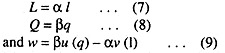
The peasants are assumed to be guided in their allocation efforts by the aim of maximising the happiness of the family. Furthermore, they know that every member of the family has a personal utility function “u”, which is a function of individual income “q” and every working member has a personal disutility function “v”, related to his individual labour” l “. The functions u and v are of same shape for everyone.

Moreover,

Each i-th person’s of family welfare “w” is given by net utility from income and effort of all members taken together, attaching the same weight to everyone’s happiness:

It is further assumed that work is equally distributed between the working members and income equally between all the members of the family. Moreover all the members have identical utility and disutility functions. Accordingly we have,

Substituting the values of q and I in (9) we get

Now, we try to find out the condition for maximization of family welfare (leaving out the odd case of w max at zero labour)

Differentiating with respect to L from 9(a)

 

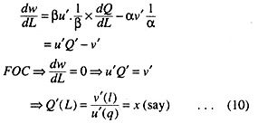
‘x’ is defined as the ‘real cost of labour’. It is given by the individual rate of substitution between income and labour. Moreover, labour is applied up to the point where its marginal product equals real cost of labour (x).

[To understand, why v'(l)/u'(q) is the real cost of labour we use unitary method.]

Now, to prove the second order condition differentiating (q) twice with respect to L, we get

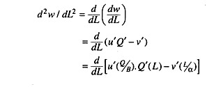
Thus we get the Soc for family welfare maximisation which satisfies the required conditions.

Thus we get,

L* (equilibrium value of labour) and maximum w for the family as well.

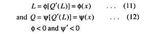
Finally, since Q”(L) < 0 throughout, L itself is a function of Q'(L), i.e., the inverse function exists. But Q'(L) equals the real cost of labour employed and also that of family output, and income can, therefore, be expressed as functions of the real cost of labour, given the equilibrium.

(ii) The Possibility of Surplus Labour and the Reduction of Peasant Output to the Working Population:

We can define surplus labour as that part of the labour force in this peasant economy that can be removed, without reducing the total amount of output produced, even when the amount of other factors is not changed. It is seen that if the reduction in the working population reduces the amount of labour put into cultivation, then there would be a reduction in the amount of output produced.

The continually diminishing marginal productivity of labour, given by equation (1), will make MP_L > 0, even if it was zero to start with, so that a smaller value of L means a smaller volume of output. Thus, what is necessary for the existence of surplus labour is that a fall in a, should be compensated by a rise in the amount of work done, per person. And this is possible only if the real labour cost is insensitive to the withdrawal of a part of the population.

The Possibility of Surplus Labour:

Equation (12) shows that a reduction in output can occur only when the real labour cost rises. Such a rise in the real cost of labour can take place for two different reasons. Firstly, an immigration of labour from the family reduces the number of working members (a) and, to maintain the same level of total family labour, each remaining member has to work longer, raising marginal disutility of labour. Secondly, a withdrawal would cause a rise in income of the remaining members of the family and, thus, reduce the marginal utility from income.

Both these effects will tend to push up Y and shift the equilibrium to a smaller volume of family labour and total output. (These conclusions will go through if we make allowance for output supply in the market and factor supply of members of peasant families). Hence the existence of surplus labour depends on the marginal utility and the marginal disutility schedules, being flat in the relevant region.

Only under that situation a rise in income would have the marginal utility unchanged and a rise in individual effort leaves the marginal disutility unaffected. Consequently, we can withdraw labour without hampering and, hence, without affecting total output and the volume of labour.

The constancy of marginal utility of income within a constant range implies an insensitivity of the usefulness of income to its quantity within this region.

Given this assumption, with suitable choice of units, we can make the constant value of marginal utility equal to unity and, hence, equilibrium changes to

Q'(L) = v'(l) = x … (13)

Now, marginal disutility of labour remains constant say z, until a certain critical amount of effort 1*, is reached:

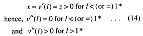
However, we assume that the withdrawal of labour in question starts in a situation when the total family labour is αl.

Now, if I > (or =) l*, there cannot be any surplus labour, if l < l*, withdrawal can take place without affecting output, i.e., surplus labour exists.

Here implicitly we assume divisibility of labour. On the other hand, if labour can only be withdrawn in units of one person, the necessary and the sufficient condition of the existence of surplus labour is given by:

⇒[the total actual family labour has to be] < (or =) [total critical amount of family effort] minus [(at least) a single individual’s critical effort].

Surplus Labour and Zero Marginal Productivity:

The existence of surplus labour is sometimes identified with the MP_L being zero. According to the above model this situation corresponds to the special case where z = 0, then the marginal disutility of labour = 0 in the relevant region.

[⇒ {z = 0 => v'(l) = 0 ⇒ Q'(L) – 0}]. However, even if MP_L > 0, it is shown that there would be the existence of surplus labour [<=> as z is a positive constant; Q'(L) = v'(l) / u'(q) = z /1 > 0, still we have surplus labour if l < l*]. Thus the constancy of real cost implies that the marginal utility schedule and the marginal disutility schedule being flat in the relevant region. Thus disguised unemployment does not require MP_L = 0. In other words, MP_L = 0 is not a necessary condition for unemployment.

Moreover, zero marginal product of labour is not a sufficient condition too. We have a situation where z = 0(⇒ MP_L = 0) but l = l* (say). In this case even if MP_L = 0, any finite withdrawal of the peasant labour force will reduce the level of output, as already the labourers are working at the capacity level.

A closely related point needs to be clarified here. It is sometimes asserted that the existence of surplus labour requires certain types of production functions with limited possibilities of facts substitutability. However, this is not the case as it is evident from the preceding analysis.

While it is true that with some production functions, for example the Cobb-Douglas or, more generally, a CES production function with positive elasticity of substitution, the MP_L never falls to zero, but this does not in any way rule out the existence of surplus labour.

At equilibrium we require that the marginal product of labour should equal the real labour of (*) and also the schedule of real labour cost should be flat but it is not necessary that the real labour cost be zero. Thus we do not have to restrict the class of production functions arbitrarily to admit the possibility of surplus labour.

In other words, specific form of production function is not necessary for the existence of surplus labour, as this existence does not depend on MP_L and, hence, could be compatible to any production function. Moreover, we have shown that surplus labour can co-exist with positive marginal productivity of labour, i.e., that marginal productivity of labour hours could be positive, while the marginal productivity of labourer is zero.

Even if the gap created by withdrawal of labourer is filled up by extra labour hour of work by each remaining labourer, MP_L (= v'(l) / u'(q) = z / 1 = z = x = real cost of labour is constant) remains constant in the relevant region. Hence we do not have any shift of the existing equilibrium family (total) labour (not labourer) and family output. Thus we get a distinction between surplus labour in terms of labour hour and that in terms of units of population, i.e., labourer.

“Thus zero marginal productivity of labour has formed the foundation for a strategy of “painless” or “up by the bootstraps” process of development (Nurkse, 1953). It is a misguided policy prescription, because, as we have seen, zero marginal productivity of labour is neither a necessary nor a sufficient condition for withdrawing workers from agriculture with a loss of output.

Sen’s result on the existence of surplus labour can be reinforced by introducing a number of assumptions as shown by Stiglitz. He showed that Sen did not consider the seasonal labour utilisation pattern. In most agricultural activities (with dairy fanning and specialised crops being the likely assumptions), the relationship between peak season labour utilisation and slack season labour utilisation is one of complementarily, rather, than substitutability.

As a result, total annual output, according to Stiglitz, is not simply a function of total labour supply, but should be taken as a function of not one homogeneous labour argument, but the labour arguments: the peak and slack season utilisations.

In the peak season, there is full utilisation of labour and demand for labour is greater than supply of labour. Therefore, L is maximum in the peak season. However, the slack season employment can be derived on the basis of utility maximisation.

With this modification, Sen’s results become even stronger. As there is a complimentarily between the slack and the peak season labour utilisations, there is not much scope of even manipulating the slack season labour usage.

Labour can never be in a surplus and total output must fall as workers migrate to the urban sector, regardless of the marginal utility of consumption and the marginal disutility of work which are crucial factor’s in Sen’s argument.

So, this observation makes the existence of surplus labour a very difficult proposition. The evidence supports Sen’s result the existence of surplus labour is also very difficult as it crucially depends on the flatness of marginal utility of income and marginal disutility of effort schedules in the relevant region.