
Here is a compilation of term papers on the ‘Supply of Goods’ for class 11 and 12. Find paragraphs, long and short term papers on the ‘Supply of Goods’ especially written for commerce students.
Term Paper on the Supply of Goods
Term Paper Contents:
- Term Paper on the Meaning of Supply
- Term Paper on the Supply Schedule, Supply Curve and Law of Supply
- Term Paper on Supply and Quantity Supplied
- Term Paper on the Changes in Supply: Increase and Decrease in Supply
- Term Paper on the Factors Determining Supply
- Term Paper on the Elasticity of Supply
Term Paper # 1. The Meaning of Supply:
As demand is defined as a schedule of the quantities of a good that will be purchased at various prices, similarly the supply refers to the schedule of the quantities of a good that will be offered for sale at various prices. To be more correct, supply of a commodity is the schedule of the quantities of a commodity that would be offered for sale at all possible prices at any moment of time or during any one period of time, for example, a day, a week and so on, the conditions of supply remaining the same.
ADVERTISEMENTS:
Supply should be carefully distinguished from stock. Stock is the total volume of a commodity which can be brought into the market for sale at a short notice and supply means the quantity which is actually brought in the market. For perishable commodities like fish and fruits, supply and stock are the same because whatever is in the stock must be disposed of.
The commodities, which are non-perishable, can be held back if prices are not favourable. In case of a non-perishable or durable commodity if the price is high, larger quantities of it are offered, by the sellers from their stock. And if its price is low, only small quantities are brought out for sale. In short, stock is potential supply.
Term Paper # 2. Supply Schedule, Supply Curve and Law of Supply:
Supply of a commodity is functionally related to its price. The law of supply relates to this functional relationship between price of a commodity and its supply. In contrast to the change in quantity demanded in response to the changes in price, the quantity supplied generally varies directly with price. That is, the higher the price, the larger is the quantity supplied.
The supply schedule or supply curve of a commodity means how price of a commodity is related to the quantity which the sellers (or producers) are willing and able to make available in the market. The supply schedule giving various prices of wheat and quantities of wheat supplied at those prices is shown in Table 4.1.

It will be seen from this table that at a price of Rs. 275 per quintal sellers are willing and able to supply 200 quintals of wheat. When the price of wheat rises to Rs. 325 per quintal, the greater quantity (300 quintals) of it is supplied in the market. If the price of wheat further goes upto Rs. 375, the still greater quantity 400 quintals are offered for sale in the market by the suppliers.
It is important to note that like the concept of demand, the concept of supply does not refer to a fixed quantity of a good which the sellers are willing and able to make available in the market. Instead, the supply of a commodity implies how the quantity supplied of the commodity varies with the change in price under the given conditions of cost and technology. Thus, supply refers to the whole schedule or curve depicting the relationship between price and quantity which the sellers produce and offer for sale in the market.
Law of Supply:
The supply schedule and supply curve reflect the law of supply. According to the law of supply, when the price of a commodity raises the quantity supplied of it in the market increases, and when the price of a commodity falls, its quantity demanded decreases, other factors determining supply remaining the same.
Thus, according to the law of supply, the quantity supplied of a commodity is directly or, positively related to price. It is due to this direct relationship between price of a commodity and its quantity supplied that the supply curve of a commodity slopes upward to right as seen from supply curve SS in Fig. 4.1. When price of wheat rises from Rs. 225 per quintal to Rs. 425 the quantity supplied of wheat in the market increases from 100 quintals to 500 quintals per period.

Why Does Supply Curve Generally Slope Upward to the Right?
The law of supply or upward-sloping supply curve implies that only at a higher price of a good, more quantity of it will be produced and made available in the market during a given period. Why at a higher price, more quantity of a good is supplied? The reason is that at a higher price of the commodity, other things remaining the same, the greater the potential profits which producers can generally expect from producing and supplying it in the market.
The law of supply and positively sloping supply curve is based upon two important assumptions. First, producers or sellers aim to maximise profits from production and sale of a commodity. Secondly, as output of a commodity is expanded, the additional cost of producing an extra unit goes up due to diminishing returns to the variable factors.
To understand why more is supplied at a higher price, during a given period, let us illustrate it with an example. Suppose the demand for ready-made shirts in a given period increases, the firms producing them cannot easily increase the factory space and machinery used in the production of ready-made shirts in the short run.
The firms will expand their output by employing more of the variable factors which can be easily increased in the short-run such as labour and cloth (which is the raw material for producing shirts), keeping other factors fixed. But the as factory-space, machinery will cause the total output of shirts to increase at a diminishing rate.
In economic terms, it is said that the diminishing marginal returns accrue to the extra units of labour and other variable factors employed to expand output to meet the increased demand for the shirts. In order to maximise profits, the producer will equate price of a product with the additional or marginal cost of producing a unit of output.
Since the marginal cost of a unit of output increases as output is expanded due to the occurrence of diminishing marginal returns to the variable factors, the producer will be willing to produce and make available in the market more quantity of a commodity only at a higher price.
It may however be noted that if diminishing marginal returns to factors do not occur and therefore marginal cost does not rise with the expansion in output as may be the case in the long run when all factors including fixed factors such as factory-space and machinery can be easily increased, the supply curve of output will be a horizontal straight line and the law of supply will not hold. Thus, it is the rising marginal cost of additional units of output coupled with the objective of maximising profits on the part of producers that explain the upward-sloping supply curve of output which reflects the law of supply.
It is important to note that each point on the supply curve indicates the price at which a given quantity of output the producers will be willing to supply, that is, make it available in the market. The price at which a given quantity of the commodity is supplied by the sellers is called supply price.
The upward-sloping supply curve indicates that the supply price increases if more quantity of the good is to be supplied in the market. Thus, the greater the quantity which the consumers would like to buy the higher the price, necessary to induce the producers to produce a commodity and make it available in the market.
Term Paper # 3. Supply and Quantity Supplied:
As in case of demand and quantity demanded, the supply should not be confused with the quantity supplied. Whereas the supply describes the whole schedule or curve depicting the relationship between price and quantity supplied in a period, the quantity supplied refers to the quantity which the producers would make it available at a particular price of the commodity.
ADVERTISEMENTS:
The quantity supplied varies with a change in price of a commodity. Thus, change in quantity supplied of a commodity occurs in response to a change in its price; at a higher price, more quantity of it is supplied and vice-versa. For example, in our illustration given above, when price of wheat rises from Rs. 225 to Rs. 425 per quintal, the quantity supplied of wheat increases from 100 quintals to 500 quintals, the supply schedule or supply curve being given.
The terms extension and contraction in supply are used for changes in quantity supplied as a result of changes in price of a commodity. When the rise in price of a commodity brings about increase in quantity supplied of the commodity, other factors determining supply remaining constant, this is called extension in supply. On the other hand, when price of a commodity falls and as a result, the quantity supplied of it decreases, contraction in supply is said to have occurred, other factors being held constant.
Thus extension in supply should be carefully distinguished from increase in supply. While extension in supply of a commodity occurs as a result of rise in price of the commodity, increase’ in supply means that due to reduction in prices of resources improvement in technology, whole supply curve shifts to the right showing more is supplied than before at each price of the commodity.
ADVERTISEMENTS:
Similarly, there is contraction in supply of a commodity when its price falls, that is, when a smaller quantity of it is supplied at a lower price whereas decrease in supply implies that because of rise in prices of resources, imposition of excise duty, etc., the entire supply curve shifts to the left so that less quantity of the commodity is supplied at every price.
Term Paper # 4. Changes in Supply: Increase and Decrease in Supply:
The supply of a commodity in economics means the entire schedule or curve depicting the relationship between price and quantity supply of the commodity, the other factors including supply remaining constant. These other factors are the state of technology, prices of inputs (resources), prices of other related commodities, etc. which are assumed constant when the relationship between price and quantity supplied of a commodity is examined.
It is the changes in these factors that cause a shift in the supply schedule or curve. Thus a change in supply refers to the shift in the supply curve due to the changes in factors other than price. For example, when prices of inputs such as labour and raw materials used for the production of a commodity decline, this will result in lowering the cost of production which will induce the producers to produce and make available greater quantity of the commodity in the market at each price. This means increase in supply has taken place.
This increase in supply of a commodity due to the reduction in prices of inputs will cause the entire supply curve to shift to the right as shown in Fig. 4.2, where the supply curve shifts from SS to S’S’. As shown by arrow marks, at prices P1, P2 and P3, quantity supplied increases when supply increases causing a rightward shift in the supply curve. Similarly, progress in technology used for production of a commodity will also cause a shift in the supply curve to the right.
ADVERTISEMENTS:

On the other hand, decrease in supply means the reduction in quantity supplied at each price of the commodity as shown in Fig. 4.3 where as a result of decrease in supply, the supply curve shifts to the left from SS to S”S”. As shown by the arrow marks, at each price such as P1, P2, and P3 the quantity supplied on the supply curve S”S” has declined as compared to the supply curve SS. The decrease in supply occurs when the prices of factors (inputs) used for the production of a commodity go up so that each quantity of the commodity is produced at a higher cost per unit which causes a reduction in quantity supplied at each price.

Similarly, the imposition of an excise duty or sales tax on a commodity means that each quantity will now be supplied at a higher price than before so as to cover the excise duty or sales tax per unit. This implies that quantity supplied of the commodity at each price will decrease as shown by the shift of the supply curve to the left.
Another important factor causing a decrease in supply of a commodity is the rise in prices of other commodities using the same factors. For example, if the price of wheat rises sharply, it will become more profitable for the farmers to grow it. This will induce the farmers to reduce the cultivated area under other crops, say sugar cane and devote it to the production of wheat. This will lead to decrease in supply of sugar cane whose supply curve will shift to the left.
Further, agricultural production in India greatly depends on the rainfall due to monsoon. If monsoon come in time and rainfall is adequate, there are bumper crops, the supply of agricultural products increases. However, in a year when monsoon are untimely or highly inadequate, there is a sharp drop in agricultural production causing a decrease in the supply of agricultural output and thereby shift the supply curve of agricultural output to the left. We thus see that there are several factors other than price which determine the supply of commodity and any change in them causes a shift in the entire supply curve.
Term Paper # 5. Factors Determining Supply:
ADVERTISEMENTS:
It is clear from the supply schedule (Table 4.1) and the supply curve (Fig. 4.2) that the quantity supplied varies directly with the price of a product. A supply schedule and supply curve show that the supply of a product is function of its price. However, the supply depends not only on the price of a product but on several other factors too.
The effect of changes in price of a product on the quantity supplied of it is explained by a movement along a given supply schedule or curve, the effect of other factors is represented by the shifts in the entire supply schedule or supply curve. While making a supply schedule or a supply curve we assume that these other factors remain the same. Thus when these other factors change, they cause a shift in the entire supply curve.
The factors other than price which determine price are the following:
(a) Production Technology:
A change in technology affects the supply function by altering the cost of production. If there occurs an improvement in production technology used by the firms, the cost of production declines and consequently the firms would supply more than before at the given price. That is, the supply would increase implying that the supply curve would shift to the right.
(b) Prices of Factors:
Changes in prices of factors or resources also cause a change in the cost of production and consequently bring about a change in supply For example, if either wages of labour increase or prices of raw materials and fuel go up, the unit cost of production will rise. With a higher unit cost of production, less would be supplied than before at various prices. This implies that supply curve would shift to the left.
(c) Prices of Other Products:
When we draw a supply curve we assume that the prices of other products remain unchanged. Now, any change in the prices of other products would influence the supply of a product by causing substitution of one product for another. For example, if the market price of wheat rises, it will lead to the reduction of the production and supply of gram by the farmers as they would withdraw some land and other resources from the production of gram and devote them to the production of wheat. This will cause a leftward shift in the supply curve of gram.
(d) Objective of the Firm:
ADVERTISEMENTS:
The objective of a firm also determines the supply of a product produced by it. If the firm aim to maximize sales or revenue rather than profits, the production of the product produced by it and hence the supply of it in the market would be larger.
(e) Number of Producers (or Firms):
If number of firms producing a product increases, the market supply of the product will increase causing a rightward shift in the supply curve. When, in the short-run, firms in an industry are making large profits, new firms enter that industry in the long-run and expand the total production and supply of the product of that industry. On the other hand, due to losses when some firms leave the industry, the supply of its product will decrease and supply curve will shift to the left.
(f) Future Price Expectations:
The supply of a commodity in the market at any time is also determined by sellers’ expectations of future prices. If, as happens during inflationary periods, sellers expect the prices to rise in future, they would reduce supply of products in the market and would instead hoard them. The hoarding of huge quantities of goods by traders is an important factor in reducing supplies in the market and thus causing further rise in their prices.
(g) Taxes and Subsidies:
Taxes and subsidies also influence the supply of a product. If an excise duty or sales tax is levied on a product, the firms will supply the same amount of it at a higher price or less quantity of it at the same price. This implies that imposition of a sales tax or excise duty causes a leftward shift in the supply curve. The opposite happens case of the supply of a commodity on which the government provides subsides.
It follows from above that technology, prices of factors and other products, expectations regarding future prices and objective of the firms are the important determinants of supply which cause rightward or leftward shift in the whole supply curve.
Term Paper # 6. Elasticity of Supply:
When a small fall in the price of a commodity leads to a large contraction in supply, the supply is comparatively elastic. But when a big fall in price leads to a very small contraction in supply, the supply is said to be comparatively inelastic. Conversely, a small rise in price leading to a big extension in supply shows elastic supply, and a big rise in price leading to a small extension in supply indicates inelastic supply.
ADVERTISEMENTS:
Consider Figs. 4.4 and 4.5 where two supply curves SS have been drawn. At price OP1, the quantity supplied in Fig. 4.4 is OQ1 and the quantity supplied in Fig. 4.5 is ON1. With rise in price of the product, quantity supplied increases from OQ to OQ2 in Fig. 4.4 and from ON1 to ON2 in Fig. 4.5.
Whereas the relative change in price- is the same in both the figures, the increase in quantity supplied Q1Q2 in Fig. 4.4 is much larger as compared to the increase in quantity supplied N1N2 in Fig. 4.5. Therefore, supply in Fig. 4.4 is said to be elastic, whereas that in Fig. 4.5 is inelastic. The elasticities of supply of various products differ very much from each other.


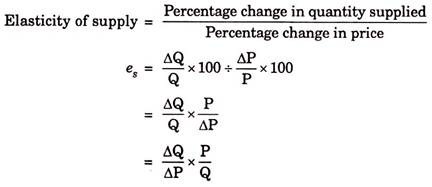
The concept of elasticity of supply, like the elasticity of demand, is a relative measure of the responsiveness of quantity supplied of a commodity to a change in its price. The greater the responsiveness of quantity supplied of a commodity to the changes in its price, the greater its elasticity of supply. In precise terms, the elasticity of supply can be defined as a percentage change in the quantity supplied of a product divided by the percentage change in price that caused the change in quantity supplied.
If the price of a refrigerator rises from Rs. 2,000 per unit to Rs. 2,100 per unit and in response to this rise in price, quantity supplied of it increases from 2,500 units to 3,000 units, the elasticity of supply.
![]()
If the supply curve of a commodity is upward sloping as is generally the case (See Figs. 4.4 and 4.5), the coefficient of elasticity of supply will have a positive sign. When the supply curve is upward sloping, the elasticity of supply will be anything between zero and infinity. When the quantity supplied of a commodity does not change at all in response to the changes in its price, the elasticity of supply is zero.
In the case of zero elasticity of supply, the supply curve will be a vertical straight line parallel to the Y-axis and is said to be perfectly inelastic (See Fig. 4.6). On the other hand, if at a price any quantity of a good can be supplied, its elasticity will be equal to infinity and its supply curve will be a horizontal straight line parallel to the quantity axis and is said to be perfectly elastic (See Fig. 4.7).


Measuring Elasticity of Supply at a Point on the Supply Curve:
Now, an important question is how elasticity of supply can be measured at a point on a given supply curve. Consider a linear supply curve SS drawn in Fig. 4.8 where we are required to measure elasticity of supply at point R on it corresponding to output OQ and price OP. In order to measure supply elasticity at point R we extend the supply curve so that it meets the X-axis at point T. Then measure of elasticity of supply at point R can be obtained by dividing the distance TQ by the distance OQ.
Thus,
Supply elasticity at point R on supply curve SS (es) = TQ/OQ.
Proof:
That the elasticity of supply at point R on the supply curve SS in Fig. 4.8 is given TQ by TQ/OQ can be easily proved as under:
es = ΔQ/ΔP. P/Q

The term ΔQ/ΔP in the elasticity formula is the reciprocal of the slope of supply curve SS (note that the slope of the supply curve is equal to ΔP/ΔQ.
Thus, rewriting the measure of the coefficient of supply elasticity we have:
![]()
Now consider Fig. 4.8. The slope of the supply curve SS is equal to RQ/TQ, price at point R is RQ and quantity supplied is equal to OQ.
Substituting these values in the formula for coefficient of supply elasticity we have:
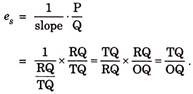
Thus elasticity of supply is given by the ratio of distance TQ and OQ.
In Fig. 4.8, the supply curve when extended meets the X-axis to the left of the point of origin, TQ is greater than OQ, elasticity coefficient TQ/OQ will therefore be greater than one.
In Fig. 4.9 supply curve when extended meets the X-axis to the right of the point of origin so that TQ is smaller than OQ. Therefore, in Fig. 4.9 the elasticity of supply TQ/OQ is less than unity. In Fig. 4.10 supply curve when extended meets the X-axis exactly at the point of origin so that TQ is equal to OQ. Therefore, in Fig. 4.10 elasticity of supply will be equal to one.
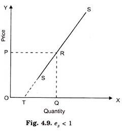
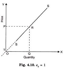
In Fig. 4.8 elasticity of supply will be greater than one at every point of the supply curve, but it will differ from point to point. Similarly in Fig. 4.9 supply elasticity is less than one at every point of the supply curve, but it will differ from point to point. However, in Fig. 4.10 elasticity of supply will be equal to one at every point of the supply curve.
Point Elasticity of Supply on a Non-Linear Supply Curve:
We have studied how the elasticity of supply is measured at a point on a straight line supply curve. But now the question is how the point elasticity of supply can be measured on a non-linear supply curve. Consider Fig. 4.11 where a non-linear supply curve has been drawn and it is required to measure elasticity at point A on it. The general principle involved is the same as derived above. In order to apply the above principle for estimating the elasticity of supply at point A on the supply curve SS, we have to draw a tangent at it. Now, a tangent t1 t1 has been drawn at point A. On being extended, tangent t1 t1 meets the X-axis at point T1.
Therefore, elasticity of supply at point A on the supply curve is = T1Q1/OQ1.

Likewise, we can find out the elasticity of supply at point B on the supply curve. For this, tangent t2 t2 has been drawn at point B and has been extended to meet the X-axis at point T2. Thus, price elasticity at point B on the supply curve SS is equal to T2Q2/OQ2. It is also evident from Fig. 4.11 that price elasticity of supply at point A and B is different. Since T2Q2/OQ2 is less than T1Q1/OQ1, price elasticity of supply at point B is less than that at A.
Factors Determining Elasticity of Supply:
Elasticity of supply plays an important role in determining prices of products. To what extent price of a product will rise following the increase in demand for it depends on the elasticity of supply. The greater the elasticity of supply of a product, the less the rise in its price when, demand for it increases.
We explain below the factors which determine price elasticity of supply of a product:
1. The Changes in Marginal Cost of Production:
Elasticity of supply of a commodity depends upon the case with which increases in output can be obtained without bringing about rise in cost of production. If with the increase in production, the marginal cost of production goes up, the elasticity of supply to that extent would be less. In the short-run, with some factors of production being fixed, the increase in the amount of a variable factor eventually causes diminishing marginal returns and as a result with the expansion of output marginal cost of production rises.
This causes supply of a commodity in the short run less elastic. However, in the long-run, the firms can increase output by varying all factors and also the new firms can enter the industry and thereby add’ to the supply of a commodity. Therefore, the long-run supply curve of a commodity is more elastic than that of the short-run.
In the increasing cost industry, that is, the industry which experience increases in cost when industry expands through the entry of new firms, the long-run supply curve, like the short-run one, is upward sloping, but will be more elastic than in a short-run. In the constant cost industry, i.e., the industry wherein there are neither net external economies and nor net external diseconomies, the long-run supply curve, as has been stated above, is perfectly elastic because in this case increases in the industrial output can be obtained at the same cost of production, that is, without raising average and marginal cost curves.
In the decreasing cost industry, that is, industry which is subject to increasing returns, long-run supply curve is downward sloping and has therefore a negative elasticity of supply. This is because in the case of decreasing-cost industry expansion in the industry brings down the cost of production and therefore additional output is forthcoming at a lower supply price.
2. Behaviour Pattern of the Producers:
Besides the change in cost of production, the elasticity of supply for a product depends on the responsiveness of producers to changes in its price. If the producers do not respond positively to the increase in prices, the quantity supplied of a product would not increase as a result of rise in its price. A profit-maximising producer will increase the quantity supplied of a product following the rise in its price.
However, producers do not always exhibit profit maximizing behaviour, as is generally assumed in economic theory and as a result do not raise supply in response to the rise in price. For example, it has been argued by some with some empirical evidence that farmers in developing countries respond negatively to the rise in price of their agricultural products. They point out that at higher agricultural prices, their need for fixed money income is met by selling smaller quantities of food-grains and therefore at higher prices they produce and sell smaller quantities rather than more.
3. Availability of the Production Facilities for Expanding Output:
The extent to which the producers would raise supply of their products also depends on the availability of productive facilities and inputs required for the production of goods. For example, when there is lack of fertilisers, irrigation facilities, the farmers would not be able to raise the supplies of agricultural products in response to the rise in their prices even if they want to do so. Likewise, in the industrial field if there is shortage of power, fuel, essential raw materials, the expansion in supply would not be forthcoming in response to the rise in prices of industrial products.
4. Possibilities of Substitution of One Product for the Others:
The change in quantity supplied of a product following the changes in its price depends on the possibilities of substitution of one product for others. For example, if market price of wheat rises, the farmers will try to shift resources such as land, fertilisers away from other products such as pulses to devote them to the production of wheat. The greater the extent of possibilities of shifting resources from the other products to wheat production, the greater the elasticity of supply of wheat.
5. The Length of Time:
The elasticity of supply of a product also depends on the length of time during which producers have to respond to a given change in price of a product. Generally, the longer the time producers get to make adjustments for changing the level of output in response to a change in price, the greater the response of output, that is, the greater the elasticity of supply.
From the viewpoint of the influence of the length of time on the elasticity of supply we distinguish between three time periods:
(1) Market period or very short run,
(2) Short run, and
(3) Long run.
In the market period no more production is possible. Therefore, market period supply curve is a vertical straight line (i.e., perfectly inelastic). In the short-run, firms can change output by changing the amounts of only variable factors; short-run supply curve is somewhat elastic. In the long run since firms can adjust all factors of production and also new firms can enter or leave the industry, long-run supply curve is more elastic.