
Here is a compilation of term papers on the ‘Laws of Consumption’. Find paragraphs, long and short term papers on the ‘Laws of Consumption’ especially written for school and college students.
Term Paper Contents:
- Term Paper on the Utility- A Basis of Consumer Demand
- Term Paper on the Law of Diminishing Marginal Utility
- Term Paper on the Cardinal and Ordinal Approaches of Utility
- Term Paper on Indifference Curves
- Term Paper on Revealed Preference Theory
Term Paper # 1. The Utility- A Basis of Consumer Demand:
Consumers demand goods and services because they derive or expect to derive utility from them. The utility a consumer expects to derive from a good or service is the basis of demand for it. In the analysis of consumer demand the term ‘utility’ connotes a specific meaning. This section explains the meaning of utility, the related concepts and the law associated with utility.
The term utility refers to satisfaction a consumer gets from the consumption of goods and services. Evidently, an individual’s demand for a good or service will be in accordance with the utility a consumer derives from the consumption of that good. Jeremy Bentham (1748 -1832) defined utility as “the subjective sensation- pleasure, satisfaction, wish, fulfillment, cessation of needs, which are derived from consuming a commodity and the experience of which is the object of consumption”. To Marshall, utility of a commodity depends on consumer’s specific relation with the commodity.
ADVERTISEMENTS:
Goods are demanded because they possess the power to satisfy human want. The more the power of a commodity to satisfy human want, the more utility the consumer has from it. Utility can, thus, be defined as the want satisfying power or capacity of a good of service.
For the simplicity of analysis it is useful to distinguish between total utility and marginal utility.
Total Utility:
Total utility (TU) is the total satisfaction a person gains from all those units of a commodity consumed within a given time period. The more units of a commodity a consumer consumes, greater will be total utility up to a certain point. As he or she goes on increasing the consumption of the commodity, he eventually reaches the point of his/her maximum satisfaction. Consumption of any further units of the commodity will lead to a decline in his/her total utility. Symbolically,
ADVERTISEMENTS:
TUn = MU1 + MU2 + MU3 + ………… MUn = ΣMU …(3.1)
where TU is total utility of n units. MU1, MU2, MU3 …. MUn represent marginal utilities of first, second and nth unit of the commodity.
Marginal Utility:
Marginal utility may be defined in more than one ways. Marginal utility (MU) is the additional satisfaction gained from consuming one extra unit within a given period of time or as the utility derived from the marginal unit consumed. In other words, marginal utility is the utility of last unit or the addition to total utility by the consumption of one additional unit of the commodity. MU thus refers to the-change in total utility (DTU) as a result of change in the quantity demanded (DQ).
ADVERTISEMENTS:
MU = ΔTU/ DQ … (3.2)
where TU = change in total utility
Q = change in quantity consumed by the unit
When n numbers of units are consumed the MU may be defined symbolically,
as MUn = TUn – TUn-1 …(3.3)
The following points about the two curves (as shown in Fig. 3.1) need be noted:
i. The MU curve slopes downward. This simply illustrates the principle of diminishing marginal utility.
ii. The TU curve starts at the origin. Zero consumption yields zero utility.
iii. The TU reaches a peak when marginal utility is zero. When marginal utility is zero, there is no addition to total utility. Total utility must be at the maximum-the peak of the curve.
ADVERTISEMENTS:
iv. Marginal utility can be derived from the TU curve. It is the slope of the line joining two adjacent quantities on the curve.
Term Paper # 2. The Law of Diminishing Marginal Utility:
Satisfaction of human wants follows the law of diminishing marginal utility. The law can be stated as, “The more we have of a thing the less we want additional increments of it, or the more we want not have additional increments of its. Marshall states the law thus. “The additional benefit which a person derives from a given increase of his stock of a thing diminishes with every increase in stock that he already has.”
In other words, as the quantity consumed of a commodity increases, the utility derived from each successive unit decreases, consumption of all other commodities remaining the same. For each commodity, diminishing marginal utility prevails. The more you have of anything, the less important to you is any one unit of it. This generalization is so certain that it expresses a universal human experience.
For the law of diminishing marginal utility to hold, certain conditions must exist. The units of the commodity must be relevantly defined e.g., a cup of tea, a bottle of soft drink, a pair of shoes etc. The units must not be excessively small or large.
ADVERTISEMENTS:
The consumer’s taste or preference must not change during the period of consumption. The consumption must be continuous. A break in continuity is necessary; the time interval between the consumption of two units must be appropriately short. The mental condition of the consumer must remain normal during the period of consumption.
If these conditions prevail, the law of diminishing marginal utility holds universally. There may be certain exceptions where the marginal utility may initially increase but eventually it does decrease. As a matter of fact, the law of marginal utility generally operates universally.
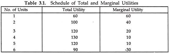
Table 3.1 numerically illustrates the law of diminishing marginal utility:
ADVERTISEMENTS:
The table shows that as the number of units consumed per unit of time increases, the total utility increases at a diminishing rate.
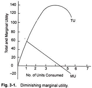
Fig. 3-1 explains the law of diminishing marginal utility. The downward sloping MU curve shows that marginal utility goes on decreasing as consumption increases. At a point total utility reaches its maximum level where marginal utility becomes zero. Beyond this level, marginal utility becomes negative and total utility begins to decline.
Term Paper # 3. Cardinal and Ordinal Approaches of Utility:
The terms cardinal and ordinal are borrowed from the vocabulary of mathematics. The numbers 1,2,3, and so on, are cardinal numbers. In contrast, the numbers 1st, 2nd, 3rd, and so on are ordinal numbers. Such numbers are ordered, or ranked, and have no way of knowing what is the size relation of the numbers. All we can know of the ordinal numbers is that the second number is greater than the first, that the third is greater than the second, and so on.
The concept of cardinality assumes that utility is quantitatively measurable. Economists who insist on using the concept of ordinal utility maintain that quantities of utility are inherently immeasurable, theoretically and conceptually as well as practically. They also maintain that many aspects of theory of consumer behavior can be explained without the idea of measurable utility. Neoclassical cardinal utility believes that utility can be measured with an arbitrary unit of measurement called utils.
Cardinal Utility Approach:
ADVERTISEMENTS:
The main theme of the consumption theory is that the consumer behaves rationally. It implies that the consumer calculates deliberately, chooses consistently, and maximizes utility. Rational behavior also can be described as behavior that results in an optimum decision.
For individuals and household consumers, the optimum is maximum attainable utility. The consumer achieves the optimum by using the best method and by making precise calculations. The rational consumer is not the only decision maker who seeks an optimum. The executive in a business corporation, in a government agency, or in a nonprofit organization also be thought of as searching for optimum decision through rational behavior.
The cardinal utility approach to consumer analysis makes the following assumptions:
Assumptions:
1. Rationality:
The consumer is assumed to be rational. He aims at the maximization of his utility subject to the constraint imposed by his given money income.
ADVERTISEMENTS:
He or she assigns the highest priority to the purchase of that commodity which yields him the highest utility and the last that gives him the least utility.
2. Cardinal Utility:
The utility of each commodity is measurable in terms of monetary units that the consumer is ready to pay for another unit of that commodity.
3. Constant Marginal Utility of Money:
The Cardinality assumes the marginal utility of money remains constant irrespective of the level of a consumer’s income. This assumption is necessary if the monetary unit is money as the measure of utility. The essential feature of a standard unit of measurement is that it be constant. If the marginal utility of money varies with income the measuring rod for utility becomes inappropriate for measurement.
4. Diminishing Marginal Utility:
ADVERTISEMENTS:
It is assumed that the marginal utility of a commodity diminishes as the consumer acquires lager quantities of it. This is the axiom of diminishing marginal utility.
5. Utility is Additive:
Cardinality assumed that utility derived from the consumption of various goods and services can be added together to obtain the total utility.
A consumer’s utility function may be expressed as,
U = f(x1, x2…..xn)…. (3.4)
Given the utility function, total utility attained from n units of a commodity may be expressed as,
ADVERTISEMENTS:
Un = U1(X1) + U2(X2) + …..Un(Xn)….(3.5)
The consumer aims to maximize this quality function.
Addition implies independent utilities, of the various commodities in the bundle. This assumption was considered unrealistic and unnecessary and therefore, dropped in later version of the cardinal theory.
Consumer’s Equilibrium:
(a) One Commodity Model:
Let us begin with the simple model of a single commodity X. We suppose that a consumer consumes only one-commodity X with his given money income. Since both money income and commodity X have utility for the consumer, he can either buy X or retain his money income Y. Under these conditions the consumer is in equilibrium when the marginal utility of X is equal to its market price (Px). Symbolically, the consumer’s equilibrium can be expressed as,
MUx = Px …(3.6)
Let us recall the assumptions that MU is subject to diminishing marginal utility, whereas marginal utility of money is assumed to remain constant. If the marginal utility of X is greater than its price, a utility maximizing consumer can increase his welfare by purchasing more units of X. Similarly if the marginal utility of X is less than its price the consumer can increase his total satisfaction by reducing the quantity of X and keep more of his income unspent.
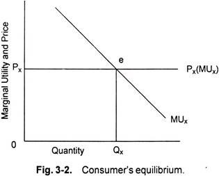
Fig. 3-2 graphically illustrates a single commodity model of consumer’s equilibrium. On the vertical axis marginal utility and price are measured. The horizontal axis measures the quantity of commodity consumed. The horizontal line Px (MUx) represents the utility of money, assumed to be constant, weighted by the price of commodity X (i.e.). MU curve shows the diminishing marginal utility of X. The Px (MUx) and MUx curve intersect each other at point e. At point e MUx is equal to Px(MUx) and OQx is the quantity consumed. Therefore, at point e the consumer is in equilibrium.
(b) Multiple Commodity Model- Consumer’s Equilibrium:
In case there are multiple commodities a consumer has to choose from how does he reach his equilibrium? In real life, however, a consumer consumes multiple goods and services.
In a multiple commodity model, the consumer’s equilibrium can be explained with the help of the law of equi-marginal utility.
The law of equi-marginal utility states that a consumer maximizes his total utility by allocating his income among goods and services available to him in such a way that the marginal utility per unit of expenditure of one good equals the marginal utility per unit of expenditure worth of any other good. In other words, a utility maximizing consumer spends his income on various goods and services he consumes in such a way that each rupee spent on each good or service yields him the same marginal utility.
Let us consider a two-commodity model. Let us suppose that a consumer consumes only two commodities, X and Y, their prices being P and P respectively.
In order to maximize total utility a consumer will distribute his income between X and Y, so that:
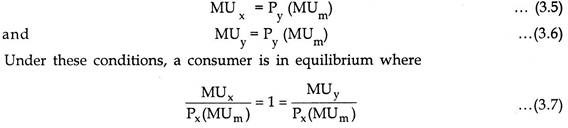
Since the marginal utility of money is assumed to be constant, the equation 3.7 can be re-expressed as,

We can conclude that the consumer attains his equilibrium when the marginal utility derived from each rupee spent on the two commodities X and Y is the same.
The two-commodity model can be generalized to explain consumer’s equilibrium for multiple commodities with given money income and at different prices.
Ordinal Utility Approach:
The Cardinal approach of consumer behavior is criticized basically for its assumption that utility is quantitatively measurable. Ordinal approach believed that measurement of subjective utility on an absolute scale is neither possible nor necessary.
Late in the nineteenth century Edgeworth realized that the assumptions of the utility theory were unrealistic. The consumer is able to rank various combinations of goods and services in order of his preference. He is in a position to tell whether he prefers one commodity bundle to another or is indifferent between them.
The preference approach to consumer behaviour emerged as a reaction to rising dissatisfaction with the Marshallian approach. Though the indifference curve approach was originally propounded by English Economist Edgeworth (1881), Italian Economist Vilfred Pare to (1906) put the indifference curve to extensive use. He took a critical step in removing the measurability assumption. His great insight pointed out that it was not necessary to assume the existence of a unique measurability utility function to obtain indifference curves.
Pareto argued that one could start with indifference curves, which in his view could be treated as a fact of experience, and derive from them directly all that was necessary for the theory of consumer equilibrium. Slutsky (1915) ,(Soviet Economist) further extended the results of Pareto.
However, the analysis received logical perfection in the hands of two English Economists R.G.D. Allen and J.R. Hicks in an article in ‘Economic’ in 1934 entitled,’ A Reconsideration of the theory of Value’. J.R. Hicks further developed the concepts in his books ‘Value and Capital'(1939) and ‘Revision in Demand Theory’ (1936).
The ordinal approach prevailed for a while, but the attack turned out to have no more effect than to tone down some of the claims for cardinal utility. The ordinal utility has its own shortcomings. Thus, both approaches coexist peacefully in economic theory.
Ordinal utility means that the consumer is able to order, or ranks the subjective utilities of goods. A consumer may prefer a ‘unit of commodity A to a unit of commodity B, and also prefers A to C. But he may have no preference between B and C, or say he is indifferent. Preference and indifference can describe the tastes of the consumer. If he chooses between two goods he prefers one to the other or else is indifferent.
Assumptions of Ordinal Utility Theory:
The Ordinal Utility Theory makes use of certain assumptions, some of which are described below:
1. Rationality:
The consumer is assumed to be rational. He aims at the maximization of his utility, given his money income and market prices with full knowledge of all relevant information.
2. Ordinal Utility:
The consumer is assumed to rank his preferences according to the satisfaction of each basket. He need not know precisely the amount of satisfaction. It suffices that he expresses his preference for the various bundles of commodities. Only ordinal measurement is required.
3. Consistency and Transitivity of Choice:
The consumer is consistent in his choice. If in one period he chooses bundle A over B, he will not choose B over A in another period if both bundles are available to him.
The consistency assumption may be symbolically expressed as under:
If A >B, the B>A
Similarly, consumer’s choices are assumed to be transitive. Transitivity of choice means that if a consumer prefers A to B and B to C, he must prefer A to C.
Symbolically, transitivity may be written as If A > B, and B > C, then A > C
4. Diminishing Marginal Rate of Substitution:
The marginal rate of substitution is the rate at which a consumer is willing to substitute one commodity for another so that his total satisfaction remains the same. The marginal rate of substitution of X for Y measures the number of units of Y that must be sacrificed per unit of X gained so as to maintain a constant level of satisfaction.
The marginal rate of substitution is the negativity of the slope of an indifference curve at a point. It is defined only for movements along an indifference curve, never for movements among curves. (Gould). The rate is given as DY/ DX. The rate goes on decreasing when a consumer continues to substitute X for Y.
5. Non-Satiety:
The consumer has not reached the point of saturation in the consumption of any good. He always prefers to have more of both commodities, and tries to move to a higher indifference curve to obtain higher and higher satisfaction.
Term Paper # 4. Indifference Curves:
An indifference curve represents satisfaction of a consumer from two commodities. It is drawn on the assumption that for all possible combinations of the two commodities, the total satisfaction remains the same. Hence, the consumer is indifferent to the combinations lying on an indifference curve.
For example, let us assume a consumer wants to buy apples and oranges and make five combinations of the two commodities, as presented in table 3.1. All these combinations yield him the same level of satisfaction.
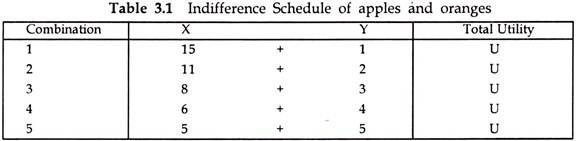
In the above schedule, the consumer obtains the same level of satisfaction from all the five combinations of apples and oranges. The combinations 1, 2, 3, 4 and 5 given in the table 3.1 are plotted and joined by a smooth curve (as shown in Fig. 3-3). The resulting curve is known as an Indifference Curve.
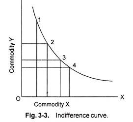
An indifference curve is a locus of points in commodity space- or commodity bundles- among which the consumer is indifferent. Each point on an indifference curve yields the same total utility as any other point on that same indifference curve.

Indifference Map:
A set of indifference curves is known an Indifference Map. Fig. 3.4 shows a set of indifference curves. An indifference map shows all the indifference curves that rank the preferences of the consumer. Combinations of goods situated on an indifference curve yield the same satisfaction. Combinations of goods lying on a higher indifference curve yield higher level of satisfaction and are preferred. Combinations of goods on a lower indifference curve yield a lower utility.
Any of the combinations on a higher indifference curve is preferable to any on a lower curve. Indifference, therefore, means sliding back and forth on any one curve, and preference means northeast to higher levels of utility. An indifference map is a collection of indifference curves corresponding to different levels of satisfaction.
Each curve on the right hand side represents a higher level of satisfaction as compared to the indifference curve on the left hand side as it represents greater quantities of both the commodities. A lower indifference curve, on the other hand, represents lesser quantities of both the commodities and hence it represents lesser level of satisfaction.
The space between X and Y axes is known as the indifference plane or commodity space. The plane is full of finite points and each point of the plane indicates a different combination of two goods X and Y. Infact, an indifference curve may contain any number of indifference curves, ranked in order of consumer’s preferences.
The Marginal Rate of Substitution:
An essential feature of the subjective theory of value is that different combinations of commodities can yield the same level of satisfaction. This means that one commodity can be substituted for another in such a way that the consumer remains on the same indifference curve.
From the indifference schedule in table 3.1 it is evident that when the consumer, in question, moves from one bundle of the two commodities to another, he is infect substituting some units of one commodity for one unit of another.
It is of considerable interest to know at which consumers are willing to substitute one commodity for another in their consumption pattern. The rate at which the substitution of one commodity for another takes place is called the Marginal Rate of Substitution. In Hick’s words, “we may define marginal rate of substitution of X for Y as the quantity of Y which would just compensate for the loss of the marginal unit of X”.
Let us consider our previous example of substitution of two commodities X and Y.
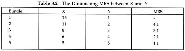
We find that when the consumer has 15 units of X and one unit of Y, he is willing to sacrifice 4 units of X for 1 unit of Y, and yet remains at the same level of satisfaction. Here the MRS of Y for X is 4:1. For the next combination, he is ready to substitute 3 units of X for an additional unit of Y.
In combination 4, he exchanges 2 units of X for 1 unit of Y, and so on. Thus, we find that as the consumer has more and more of one commodity, he is prepared to forgo less and less of the other. It can be said that the marginal rate of substitution of X for Y falls as the consumer has more of Y and less of X. Fig.3.5 explains the diminishing rate of marginal substitution.
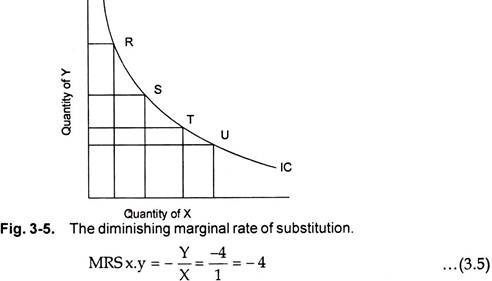
As the consumer moves down from point S to T, he loses 3 units of Y for additional unit of X, giving MRSx.y = – Y/ X = -3/1 = -3. The MRSx,y goes on diminishing as the consumer moves further down along the indifferent curve from point T to U. The diminishing marginal rate of substitution causes the indifference curves to be convex to the origin.
The reason for diminishing MRS is explained by the fact that no two goods are perfect substitutes for one another. If X and Y, for instance were perfect substitutes for each other, the indifference curves will result in a straight line with a negative slope and constant MRS.
Since the commodities are not perfect substitutes when the quantity of one commodity Y decreases and that of X increases, the marginal utility of Y increases and that of X decreases. Therefore, the consumer exchanges additional unit of Y for decreasing units of X. As a result the MRS decreases.
Properties of Indifference Curves:
Indifference curves have certain characteristics that reflect assumptions about consumer behavior. In fact, one of the major uses of indifference curves is to examine the kinds of consumer behavior implied by different preferences, prices and income.
The indifference curves have the following four basic characteristics:
1. Indifference Curves Slope Downward to the Right:
An indifference-curve slopes downward from left to right and has a negative slope. Hicks says that so long as each commodity has a positive marginal utility, the indifference curve must slope downward to the right. The negative slope of the indifference curve denotes that the two commodities can be substituted for each other and that if the quantity of one commodity Y increases, the quantity of the other (X) must decrease, if the consumer is to stay on the same level of satisfaction.
If the quantity of the other commodity does not decrease simultaneously, the bundle of commodities will increase as a result of increase in the quantity of one commodity, and a larger bundle of commodities is bound to yield a higher level of satisfaction.
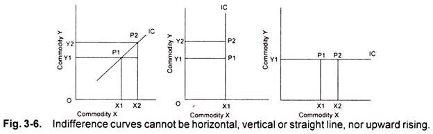
Other possibilities for the shape of an indifference curve, horizontal, vertical and upward sloping are shown in Fig.3-6. They are ruled out on the ground, as these will imply different levels of satisfaction at different points on the curve. In all the three situations, the level of satisfaction rises as the consumer moves from PI to P2. Since, he consumes more of at least one commodity with such movement. Therefore, the indifference curve slopes downward to the right.
2. Indifference Curves do not Intersect Each Other:
If the two indifference curves intersect each other, a consumer’s preferences would not be consistent or transitive. Transitivity means that if the consumer prefers A to B and B to C, he or she also prefers A to C. If the consumer is indifferent between A and B, and between B and C, the consumer must also be indifferent between A and C.
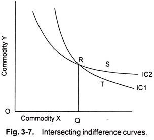
Fig. 3-7 portrays what happens when two indifference curves IC1 and IC2 intersect each other at point R. Point R lies on both the indifference curves which means that the same bundle of commodities OQ of X and RQ of Y yields different levels of satisfaction as this combination lies on two different indifference curves.
Let us take two more points S and T on IC2 and IC1 respectively. Points R,S,T represent three different combinations of X and Y. Combination R is common to both the curves as the two curves intersect at point R implying that in terms of satisfaction.
R = S
R = T
Therefore, S = T
This is inconsistent as S and T are on different indifference curves and represent different levels of satisfaction.
3. A higher indifference curve represents a higher level of satisfaction than a lower indifference curve.
An indifference curve close to the origin represents small combinations of two commodities and one farther from the point of origin represent larger combination. An indifference curve placed above and to the right of another represents a higher level of satisfaction than the lower one.
4. Indifference curves are convex to the origin.
Convexity implies that the slope of an indifference curve decreases as we move along the curve from the left downward to the right. It also implies that the marginal rate of substitution of the commodities is diminishing. The upper end of the curve shows a lot of Y and relatively little of X.
If the consumer gains X, he is ready to give up a lot of Y in order to remain on the same level of satisfaction as before. But down at the lower end of the curve, there is relatively little of Y and a lot of X. If down here the consumer gains x2 for a less amount of y, y2 will be given up by the consumer to stay on the same level of satisfaction.
Thus the convex shape of the indifference curve reflects differences in consumer feelings about giving up Y to get more X, depending on how much X and Y are already being consumed.
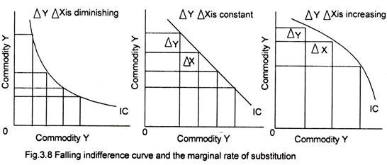
The first diagram shows the diminishing rate of marginal substitution. Besides that, we can think of two other theoretical possibilities of the trend of change in the marginal rate of substitution. It may remain the same or it may increase as we move along the indifference curve. In the central diagram, the indifference curve is a straight line.
A straight-line indifference curve shows perfect substitutes on the X and Y axes; therefore, the marginal rate of substitution remains the same in spite of the fact that the stock of one commodity continues to increase and that of other diminishes with the consumer.
The extreme end diagram the indifference curve is concave to the origin. As we move down along the curve the rate of substitution of one commodity for the other continues to increase. Therefore, the indifference curves are convex to the origin.
Budget Line and Prices:
The indifference map provides merely a hypothetical ranking of various combinations. A consumer is unable to buy a particular bundle of goods merely on the basis of indifference curves. The indifference curves do not ask the consumer which combination will give him the most for his money.
In order to study and predict the consumer behavior vital information essential in addition to the well-defined preference pattern of the consumer is the income of the consumer and the prices of the commodities. Price line or budget line shows all the combinations of the two commodities that the consumer can buy by spending his entire income for the given prices of the two commodities.
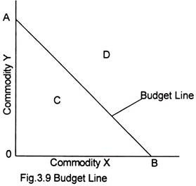
Fig. 3.9 shows how budget line is drawn. Suppose a consumer has Rs.200 to be spent on two commodities X and Y. If the price of X is Rs.20 per unit and that of Y is Rs.10 per unit, the consumer can buy 10 units of X or 20 Units of Y, when the entire income is spent. The consumer can also choose any other combination on the joining line A and B, when he partly spends his income on one commodity and partly on the other. Straight line AB is called the Budget line or Price Line.
The Budget Line suggests that the consumer cannot choose any combination of commodities beyond this line (point D), as his income does not permit him to do so. Any combination below the budget line (point C) indicates that his entire income is not spent and so his satisfaction is not maximized. The budget line is also called the consumption possibility line as it represents the different possibilities of the two goods, the consumer can purchase with his given income.
Shifting the Budget Line:
The budget line shifts upward or downward or swivels due to changes in the prices of the commodities and the consumer’s income. If the consumer’s income increases, prices of commodities remaining constant, the consumer can now purchase more of Y, more of X, or more of both.
Since prices remain constant, the slope of the budget line does not change. Thus an increase in money income, prices remaining constant, shifts the budget line upward and to the right. Since the slope does not change, the movement might be called a “parallel” shift.
A decrease in money income is shown by a parallel shift of the budget line in the direction of the origin. On the other hand, if the prices of commodities change, income of the consumer remaining the same, the budget line changes its position.
Fig. 3.10 (a) shows that given the prices of commodities X and Y and the money income of the consumer AB is the budget line. When the income of the consumer increases the budget line shifts upward to the right and the new budget line is A’B’ showing different combinations of more of both the commodities.
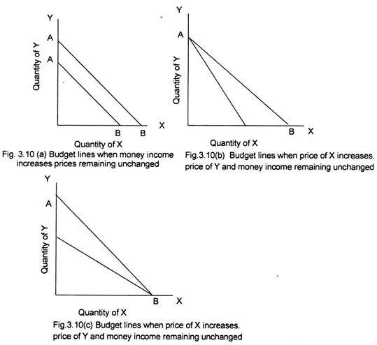
Fig. 3.10 (b) shows a shift in the budget line when the price of X increases, the price of Y and money income of the consumer remaining constant. When, the price of X increases, given money income can buy less of X. The slope of the budget line becomes steeper. Thus rotating the budget line clockwise around the ordinate intercept shows an increase in the price of X. A counter-clockwise movement represents a decrease in the price of X.
Similarly a change in the price of Y, price of X and money income of the consumer remaining constant may be treated. A rise in the price of Y rotates the budget line counterclockwise around the X-axis intercept. This is shown in fig. 3.10 (c) as the movement from AB to A’B.
Critique of Indifference Curve Analysis:
By the use of indifference analysis it has been possible to demonstrate the logical of ‘rational’ consumer choice, the derivation of the individual’s demand curve, and the income and substitution effects of a price change. All this has been done without having to resort to measuring utility.
The indifference-curves analysis has been a major advance in the field of consumer’s demand. The methodology of indifference curve has provided a framework for the measurement of the ‘consumer’s surplus’ which is important in welfare economics and in designing government policy. The analysis also provides a criterion for the classification of goods into substitutes and complements.
Nevertheless, there are limitations of indifference analysis:
1. In practice it is virtually impossible to derive indifference curves, since it would involve a consumer having to imagine a whole series of different combinations of goods and deciding in each case whether a given combination gave more, equal or less satisfaction than other combinations.
2. Consumers may not behave rationally and hence may not give careful consideration to the satisfaction they believe they will gain from consuming goods.
3. Indifference curves are based on the satisfaction that consumers believe they will gain from a good. This belief may well ‘be influenced by advertising. Consumers may be disappointed or pleasantly surprised, however, when they actually consume the good. In other words, consumers are not perfectly knowledgeable. Thus the ‘optimum consumption’ point may not in practice give consumers maximum satisfaction for, their money.
4. The approach has retained most of the weaknesses of the cardinal school with the strong assumption of rationality and the concept of the marginal utility implicit in the definition of the marginal rate of substitution.
5. Certain goods are only purchased every now and again, and then only one at a time. Such goods include consumer durables like cars, televisions and washing machines. Indifference curves are based on the assumption that marginal increases in one good can be traded off against marginal decreases in another. This will not be the case with consumer durables.
6. The indifference curve approach does not analyze the effects of advertising, of past behavior, of stocks, of the interdependence of the preferences of the consumers, which lead to behavior that would be considered as irrational, and hence is ruled out by the theory. Furthermore speculative demand and random behavior are ruled out. Yet these factors are important for the pricing and output decisions of the firm.
Term Paper # 5. Revealed Preference Theory:
The revealed preference theory states that the consumer is supposed to reveal the nature of his preferences. He exhibits the goods he would prefer to purchase in a given situation even though he may not be able to show his scale of preferences on an indifference map.
The theory of revealed preference assumes that the consumers can describe their preferences on indifference maps. The theory of revealed preference assumes that the consumer is a rational being that seeks to maximize his satisfaction from the available resources.
As such he chooses a combination of good he considers most satisfying. In one set of market conditions, he selects one combination and his choices will be different under different market situations. The choices of the consumers are consistent and transient.
The consistency implies that if a particular combination of goods P is better than Q combination and Q is better than R, then P must also be assumed to be better than R, and R cannot be better than P. Transitivity ensures that there should be no such circular relationship. The theory also assumes that the income elasticity of demand of the consumer must always be positive.
If the income of the consumer increases, his demand for the commodity must also increase. The revealed preference theory also assumes strong ordering. In a strong ordering, each item in a consumer’s scheme of purchases is assigned a definite place or number and at each number there is only one item so that the consumer definitely reveals his preferences.
In other words, choice reveals preference, by choosing one combination of goods and rejecting others, the consumer has shown his definite preference.