1. Optimisation in Managerial Decision Making:
Managerial economics is concerned with decision making by managers of a firm.
Managers of a firm have to take decisions regarding the level of output of a product to be produced, the price for a product to be charged, the size of the sales force to be engaged, the technique to be used for the production, the level of advertising expenditure to be incurred and many other such things.
In business decisions making a large number of options are open to a manager from which he has to make a choice.
Obviously, a manager will try to make a best choice from among different options available to him. A best or optimum choice is one that best achieves the desired goal or objective of the firm. For example, a manager might consider what level of output of a product he should produce.
ADVERTISEMENTS:
Manager will produce the level of output which maximises firm’s profit if he has set before himself the objective of profit-maximisation. This is a maximisation problem which he has to solve. Similarly, he may be considering choosing among the various combinations of factors or inputs that can be used for producing a level of output.
To maximise profits he will choose the combination of inputs that minimises cost for producing a given level of output. Evidently, this is a minimisation problem which he has to solve.
Decision making that involves solving of maximisation and minimisation problems is called optimisation. Therefore, for making efficient decision it is necessary for a successful manager to learn the techniques of optimisation. It may however he noted that popular techniques of optimisation are mathematical in nature. In recent year the use of analytical models of business decision making has increased the importance of the knowledge of techniques of optimisation for the students of business management.
Mathematical formulations of these analytical models of managerial decision-making are expressed in terms of functions which describe economic relationship between various variables.
ADVERTISEMENTS:
Therefore, to begin with we will explain the concept of a function and its various important types.
2. Functions:
A function describes the relation between two or more than two variables. That is, a function expresses dependence of one variable on one or more other variables. Thus, if the value of a variable Y depends on another variable X, we may write
Y = ƒ(X) (1)
Where ƒ stands for function.
ADVERTISEMENTS:
This expression (1) is read as ‘Y is function of X’. This implies that every value of the variable Y is determined by a unique value of the variable X. In the function (1), Y is known as the dependent variable and X is the independent variable. Thus in function (1) Y is called the dependent variable and its value depends on the value of X.
Further, the independent variable is interpreted as the cause and the dependent variable as the effect. An important function which is extensively used in economics is a demand function which expresses quantity demanded of a commodity is a function of its price, other factors being held constant. Thus, demand for a commodity X is described as under
Dx = ƒ(Px)
Where Dx is the quantity demanded of commodity X and Px is its price.
Similarly, supply function of a commodity X is expressed as
Sx = ƒ(Px)
When the value of the variable Y depends on more than two variables X1,X2……………………………… Xn this function is written in general form as:
Y = ƒ (X1, X2, X3, X4……………………………………………… Xn)
This shows the variable Y depends on several independent variables X1,X2,……………………………. Xn
ADVERTISEMENTS:
where n is the number of independent variables. Again note that in economics we write ’causes’ as the independent variables and ‘effect1 as the dependent variable.
For example, demand for a product is generally considered to be a function of its own price, prices of other commodities (which may be substitutes or complements), income of the consumers, tastes and preferences of the consumers and advertising expenditure made by a firm to promote its product. Thus,
Dx = ƒ(Px,Py, M, T,A)
Where
ADVERTISEMENTS:
Dx = demand for the commodity X
Px = price of the commodity X.
Py = price of a substitute product Y.
M = income of the consumers
ADVERTISEMENTS:
T = tastes and preferences of the consumer for the product.
A = advertising expenditure incurred by the firm.
The exact nature of relation of dependent variable with the independent variables can be known from the specific form of the function. The specific form of a function can take a variety of mathematical forms.
We explain below some specific types of functions:
1. Linear and Power Functions:
A widely used mathematical form of a function is a linear function.
A linear function can be stated in the following general form:
ADVERTISEMENTS:
Y = a + bX
Where a and b are positive constants and are called parameters of the function. Note that parameters of a function are variables that are fixed and given in a specific function. The values of constants a and b determine the specific nature of a linear function. The linear demand function with price as the only independent variable is written as
Qd = a-bP
The minus sign before coefficient b indicates that quantity demanded of a commodity is negatively related with price of the commodity. That is, if price of a commodity falls, its quantity demand increases and vice versa. If a equals 7 and b equals 0.5, the linear demand function can be expressed in the following specific form:
Qd = 7 – 0.5 P
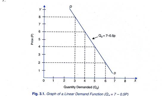
The above specific demand function shows that a unit fall in price the commodity will cause o.5 units increases in the quantity demands of the commodity .If price (P) is zero , the second term (0.5P) in the demands functions drops out the quantity demanded is equal to 7.
We can take various values of P and find out different quantities (Qd) of a commodity demanded at them. In Figure 3.1 we have plotted these price-quantity combinations on a graph and have obtained demand curve DD of the commodity representing the given demand function (Qd = 7 – 0.5P).
It should be noted that, contrary to mathematical practice, by convention in economics to represent demand function we show the independent variable (price in the above case of demand function) on the y-axis and the dependent variable (the quantity demanded in the present case) on the x-axis. Graph of linear demand function is shown in Figure 3.1. It is worth noting that slope of the demand function curve in Figure 3.1 will represent ∆P/∆P. However, if we represent quantity demanded (Qd) on the y-axis, and price (Px) on the x-axis the slope of the demand curve so drawn would be equal to ∆Q/∆P.
2. Multivariate Linear Demand Function:
Linear demand function with more than one independent variables, can be written in the following way :
Qx = a + b1 Px + b2 Py + b3 M + b4 T + b5 A
Where b1, b2, b3, b4 are the coefficients of the respective variables. In economics the effect of variables other than the own price of a commodity in the demand function are depicted by shifts in the demand curve. For instance when income (M) of the consumers increases consumers will demand more of the product X at a given price. This implies shifting of the demand curve to the right.
ADVERTISEMENTS:
The linear multivariate function is written in the following form:
Y = 4 – 0.4X1 + 0.2X2 + O.3X3 + 0. 5 X4
In this function the coefficients 0.4, 0.2, 0.3 and 0.5 show the precise impact of the independent variables X1, X2, X3, X4 on the dependent variable Y.
3. Power Functions:
The linear functions stated above are known as first degree functions where the independent variables X1, X2, X3, etc are raised to the first power only. We now turn to explain power functions. In economics power functions of the quadratic and cubic forms are extensively used.
4. Quadratic Functions:
In quadratic function one or more of the independent variables are squared, that is, raised to the second power. Note that power is also referred to as exponent. A quadratic function may be written as
ADVERTISEMENTS:
Y=a + bX + cX2
This implies that value of the dependent variable Y depends on the constant a plus the coefficient b times the value of the independent variable X plus the coefficient c times the square of the variable X. Suppose a = 4, b = 3 and c = 2 then quadratic function takes the following specific form.
Y = 4 + 3X + 2 X2
We can obtain the different values of Y for taking different values of the independent variable X.
Quadratic functions are of two types:
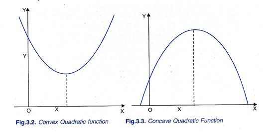
Convex quadratic functions and Concave quadratic functions. The form of quadratic function depends on the sign of the coefficient c of X2. The quadratic function, Y = a + bX + cX2, where the coefficient c of X2 is positive (i.e. c > 0) is called convex quadratic function, because its graph is U-shaped as shown in Figure 3.2. On the other hand, if coefficient of X2 is negative (c < 0), that is, when Y = a + bX- cX2, then we have concave quadratic function because its graphs is of inverted U- shape (i.e. reshaped) as shown in Figure 3.3.
It is worth noting that slope of the curve of convex quadratic functions as is evident from U-shaped graph in this case where coefficient of X2 is positive, slope is increasing everywhere. On the other hand, in case of concave quadratic function where coefficient of X2 is negative (c < O), slope of its graph is decreasing everywhere.
It should be further noted that in analytical geometry it is proved that graph of any quadratic function is a parabola which may be either convex or concave. A parabola is a curve which has a turning point and unlike the curve of a linear function, its slope is changing at different values of X.
5. Multivariable Quadratic Function:
When there are more than one independent variable such as X1, X2, and they have a quadratic relationship with the dependent variable Y, such a function, is called multivariable quadratic function.
In case of two independent variables X1 and X2 such a function may be expressed as under:
Y = a + bX1 – cX21 + dX2 – eX22
If such a function is graphically shown, it will be represented by a three – dimensional surface and not a two dimensional curve.
6. Cubic Function:
A cubic function is the power function in which there is a third degree term relating to an independent variable. Thus, cubic functions may have first degree, second degree and third degree terms.
A cubic function may have the following form:
Y=a + bX + cX2 + dX3
a is the intercept term, the dependent variable X has the first degree, second degree and third degree terms. When the signs of all the coefficients a, b, c and d are positive, then the values of V will increase by progressively larger increments as the value of X increases.
However, when the signs of various coefficients differ in the cubic function, that is, some have positive signs and some have negative signs, then the graph of the function may have both convex and concave segments depending on the values of the coefficients.
Such a cubic function where signs of the coefficients of variables differ may be expressed as follows:
Y = a + bX – cX2 + dX3
In which the sign of the coefficient c of variable X2 is negative whereas the coefficients of others are positive.

