Static Stability: Definition and Conditions (Walras)

In this article we will discuss about the definition and conditions for static stability. 

Definition of Static Stability:

In Fig. 4.1, the market equilibrium is obtained at the point E₀ (p₀, q₀). Suppose now that the market is disturbed by a rightward shift of the demand curve from D₀D₀ to D₁D₁. Because of this disturbance, quantity demanded (q^d) becomes larger by the amount E₀T than the quan­tity supplied (q^s) at the initial equilibrium price p₀, and an adjustment process would begin.

In the static analysis of stability, only consider whether the adjustment process would take the market to a new equilibrium or not.

For example, in Fig. 4.1, as the demand curve shifts and as q^d becomes larger than q^s at p = p₀, the buyers would raise their bids and price would be moving up, and, as this happens, demand would be decreasing along the D₁D₁ curve from the point T to the point E₁ and supply would be increas­ing along the S₀S₀ curve from the point E₀ to the point E₁.

The point E₁ (p₁q₁)being the point of intersec­tion between the demand curve, D₁D₁ and the supply curve, S₀S₀, would be the new equilib­rium point. If, because of a disturbance on the demand side or supply side of the market, the market moves (does not move) from an initial equilibrium to a new equilibrium, then it can be said that the equilibrium is stable (unstable) in the static sense.

Conditions for Static Stability (Walras):

The conditions for static stability can be obtained.

Suppose, the demand and supply functions for a good are:

q^d = q^d(p) …..(4.1)

and q^s = q^s(p) …..(4.2)

Therefore, the market equilibrium condition is:

q^d(p) = q^s(p) ……(4.3)

Next, define the excess demand, E, at price p to be the difference between q^d and q^s at price p, i.e.,

It can be written as:

E(p) = q^d(p)-q^s(p) …….(4.4)

The Walrasian stability condition is based on the behavioural assumption that the buyers would tend to raise their bids if E is positive and the sellers would tend to lower their prices if E is negative. If this assumption is correct, then a market is stable if E diminishes (increases) as the price of the good rises (falls), i.e., if

The reasoning that takes us to the stability condition (4.5) is this:

If the market is disturbed and E(p) becomes positive, i.e., q^d > q^s, then the buyers would raise their bids and the price would rise. The market stability, i.e., restoration of E(p) _p= 0, requires that as p rises, E must fall to become zero eventually.

On the other hand, if E(p) becomes nega­tive, i.e., q^d < q^s, the sellers would lower their prices and p would be falling. Here E(p) = 0 would be ob­tained, eventually, if E (= negative) increases as p falls. That is, market stability requires a negative relation be­tween p and E(p), as is given in (4.5).

In Fig. 4.1, p is measured along the vertical axis and, q^d and q^s are measured along the horizontal axis. That is why, here, the demand and supply curves represent the inverses of the demand and supply functions (4.1) and (4.2) and so, the slopes of the de­mand and supply curves would be, respectively, the reciprocals of (q^d)’ and (q^s)’.

 

 

 

 

 

 

 

 

 

 

In Fig. 4.2, both the demand and supply curves are positively sloped, and the former is steeper than the latter, i.e., condition (4.5) or (4.6) has been satisfied.

Here a rightward shift in the demand curve would lead to a positive excess demand = E₀T which, again, would give rise to a rising price and a falling excess demand. Eventually, at p = p₁, again reach a new equilibrium at the point E₁ (p₁q₁). Hence, it is a case of stable equilibrium.

On the other hand, if both the demand and the supply curves are positively sloped, and the supply curve is steeper than the demand curve as has been shown in Fig. 4.3, then condition p (4.5) or, (4.6) would not be satisfied. In this case, any disturbance at the initial equilibrium point would make the system unstable—it would never come back to an equilibrium position.

In Fig. 4.3, initially, equilibrium occurs at the point E₀ (p₀, q₀). Suppose now that equilibrium is dis­turbed by a rightward shift in the supply curve from S₀S₀ to S₁S₁. As a result, there would be an excess supply of E₀T which would make the sellers willing to lower their prices.

But, as the price of the good comes down, the supply and the demand curves (S₁S₁ and D₀D₀) would drift away from each other and they would never meet, i.e., equilibrium would never come back. Hence, it is a case of unstable equilibrium.

In Fig. 4.3, it is seen that if the price could somehow go up from P₀ to p₁, the market equilibrium might have been restored at the point Ep But the (assumed) behaviour of the buyers and sellers would prevent that occurrence.

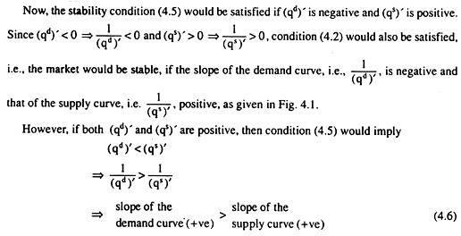
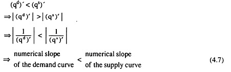
Again, if (q^d)’ and (q^s)’ are both negative, then 1/(q^d)’ and 1/(q^s)’, would be both negative, i.e., both the demand-and supply curves would be negatively sloped, then condition (4.5) would imply

 

 

 

 

 

 

Condition (4.7) gives that, in this case of negative demand and supply curves, stability requires that the demand curve should be flatter than the supply curve like those shown in Fig. 4.4. Here, initially, equilibrium occurs at the point E₀ (P₀, q₀) and a shift rightward of the demand curve from D₀D₀ to D₁D₁ causes the emergence of excess demand of the amount E₀T.

This makes the buyers raise their bids and the price would go up. As price increases from p₀ to P₁, equilibrium is restored at the point E₁ (p_1` q₁). Hence, it is a case of stable equilibrium.

However, if both the demand and supply curves are negatively sloped, and the former is steeper than the latter as is the case in Fig. 4.5, then condition (4.7) would not be satisfied and the market would be unstable.

In Fig. 4.5, initially, the market equilibrium occurs at the point E₀(p₀, q₀) and a rightward shift of the demand curve would result in an excess demand of the amount E₀T. This makes the buyers raise their bids, and the price would go up. But in Fig. 4.5, as the price goes up from p₀, the demand and the supply curves D₁D₁ and S₀S₀ would drift away from each other never to meet again. Hence equilibrium here is unstable.

In Fig. 4.5, it is seen that if the price could somehow decrease from p₀ to p₁, the market equilibrium might have been restored at the point E₁, But the behaviour of the buyers and sellers would prevent that occurrence.

Lastly, if (q^d )’ is positive and (q^s)’ is negative, then 1/(q^d)’ or the slope of the supply of curve would be positive and 1/(q^s)’ or the slope of the supply curve would be negative as in Fig. 4.6. In this case, con­dition (4.5) would not be satisfied and the market would be unstable.

In Fig. 4.6, initially, the market equilibrium occurs at the point E₀ (p₀, q₀) and a rightward shift of the demand curve from D₀D₀ to D₁D₁ gives rise to an excess demand of E₀T.

This would make the buyers raise their bids and the price would go up from p₀. But as price in­creases, the demand and supply curves, D₁D₁ and S₀S₀, move away from each other and equilibrium will never restored.

Hence, it is a case of unstable equilibrium. It is seen in Fig. 4.6 that if price could somehow come down from p₀ to p₁ the market equilibrium might have been obtained at the point E₁. But the behaviour of the buyers and sellers would not let that happen.