Notes on Dynamic Stability | Market Equilibrium

The below mentioned article provides notes on the dynamic stability of market equilibrium.

Market equilibrium is stable in the dynamic sense if the price converges to the equilibrium price over time; it is unstable if the price moves away from the equilibrium over time. The dynamic analysis of the stability of equilibrium tries to find out the course of price over time.

The Walrasian behaviour assumption that a positive excess demand tends to raise price can be expressed in terms of the following equation:

P_t − P_t−1 = kE(P_t−1) …….(4.8)

where p_t and p_t−1 are the prices in periods t and t – 1, respectively, and k is a positive constant. Equation (4.8) ensures that if there is a positive excess demand, E(p_t−1), in period (t−1), then the buyers would bid a price p_t = p_t−1 + kE (p_t−1) > p_t−1 in the following period, i.e., period t.

Assume that the demand and supply functions are:

D_t = ap_t + b ……..(4.9)

S_t = Ap_t + B ……..(4.10)

and, therefore, the market equilibrium condition is

D_t = S_t …….(4.11)

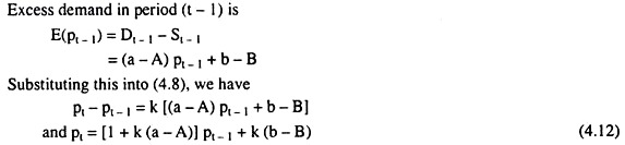
(4.12) is a first-order difference equation. It describes the time-path of price on the basis of the behaviour assumption contained in (4.8).

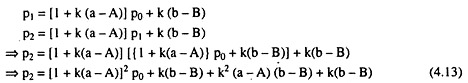
Given the initial condition p = p₀ when t = 0, the solution can be obtained from eqn (4.12) with the help of the method of iteration in the following way:

Now, the summation of the 2nd, 3rd and 4th terms of the right hand side of (4.13) is:

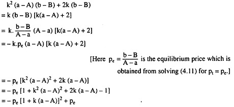
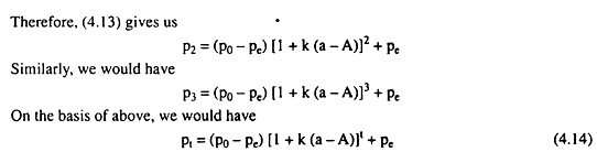
(4.14) gives us the solution of difference equation (4.12). In eqn (4.14), p_e =b-B/A-a is the market equilibrium price. Eqn. (4.14) shows us that the equilibrium is stable, if the actual price level, p_t, approaches p_e as t increases. The price level converges to p_e without oscillations if 1 + k(a − A) is positive and less than one, i.e.,

0 < 1 + k (a – A) < 1 ………….(4.15)

The right hand side of inequality (4.15) holds if:

a < A ……….(4.16)

The left hand side holds if:

k< 1/A−a ……(4.17)

Now, condition (4.16) is automatically fulfilled if the supply function has positive slope (A > 0) and the demand function has negative slope (a < 0). In this case, conditions (4.16) and (4.17) together imply that 1+ k(a − A) would be positive and its magnitude would be less than one.

(4.14) then would give us that the price level, p_t, would move upwards over time to approach p_e if the initial price p₀ is less than the equilibrium price, p_e. On the other hand, if p₀ > p_e, the price level, p_t, would move downwards over time to approach the equilibrium price p_e. On the other hand, if both the demand and supply curves are negatively sloped (i.e., if both a and A are negative), stability condition (4.16) would require

i.e., the numerical slope of the demand curve should be less than that of the supply curve, i.e., the demand curve should be flatter than the supply curve. Here, condition (4.16) along with condition (4.17) gives us that 1 + k(a − A) would be positive and less than one. This would imply that if p₀ ≶ p_e, the price level, p_t, would move upwards/downwards over time to ap­proach the equilibrium price, p_e.

However, if the slopes of both demand and supply curves are negative and the demand curve is steeper than the supply curve, i.e., if a > A, then 1 + k(a − A) > 1.

Therefore, in this case, as t increases, p_t would become smaller and smaller than P_e or larger and larger than p_e according as p₀ < p_e or p₀ > p_e. That is, when demand and supply curves are both negatively sloped and the former is steeper than the latter, market equilibrium would be unstable.

Lastly, if a − A is negative and k is sufficiently large to make 1 + k(a − A) also negative, the price level, p_t, would oscillate over time—it would be above or below the equilibrium price, p_e, in alternative periods.

If p₀ < p_e, then p_t − p_e would be positive, i.e., p_t > p_e in all odd-ordered periods like t = 1, 3, 5………. and p_t − p_e would be negative, i.e., p_t < p_e in all even-numbered periods like t = 2, 4, 6, … On the other hand, if p₀ > p_e, then p_t − p_c would be negative, i.e., p_t < p_e in all odd-numbered periods and p_t – p_e would be positive, i.e., p_t > p_e in all even- numbered periods.

If 1 + k(a − A) is negative and its magnitude is less than one, i.e., if- 1 < 1 + k(a − A) < 0, the amplitude of the oscillations decreases over time (i.e., as t increases), and the time path approaches the equilibrium level. On the other hand, if 1 + k(a − A) is less than −1, the market would be unstable, being subject to increasing fluctuations of price.

In the above analysis, it is seen that both static and dynamic stability depend upon the slopes of the demand and supply curves. Dynamic stability, in addition, depends upon the magnitude of the parameter k, which indicates the nature of market adjustments to discrepancies between the quantities demanded and supplied per period.

A large k indicates that buyers and sellers tend to “over-adjust”—if there is excess demand in one period, the buyers would overreact in increasing their bids so that price would overshoot the equilibrium price, and, there being excess supply in the next period, price would come down towards the equilibrium level but, again, it would overshoot.

That is, each adjustment would be in the right direction, but its magnitude would be more than what is needed. Thus the dynamic analysis considers also the strength of reactions to disturbances.