Demand and Marginal Utility (With Diagram) | Indifference Curve

Read this article to learn about: 1. Subject-Matter of Demand and Marginal Utility 2. Marginal Utility and Total Utility 3. Diminishing Marginal Utility 4. Demand Curve 5. Indifference Curve Analysis 6. Indifference Curves 7. Indifference Curves Slope Downwards from Left to Right and other things.

Demand and Marginal Utility # 1. Subject-Matter:

We will analyse more closely the theory of why individuals or households spend their money as they do in this article.

There are two major approaches of consumer behaviour that are available, but neither presents a complete picture.

The first approach is the marginal utility or cardinalist approach.

Secondly, we get out ordinalist or indifference curve approach. At the end of this section we shall consider Samuelson’s revealed preference approach.

Demand and Marginal Utility # 2. Marginal Utility and Total Utility:

The Law of Diminishing Marginal Utility States:

Other things being constant, as more and more units of a commodity are consumed, the additional satisfaction or utility derived from the consumption of each successive unit will decrease. This is only true if all other factors such as income, time, etc. remain unchanged.

In the 19th century, many economists, including Marshall, believed that it was possible for utility to be measured in cardinal numbers. Hence, these economists are termed cardinalists. For example, we might say that a consumer derives 20 utils of utility from consuming the first unit of a commodity, 18 utils from the second, and so on.

In fact, it is impossible to measure utility in this manner since it is a matter of subjective judgment as to how much utility a person is deriving from his consumption.

However, we will follow this approach a little further and learn something from it.

Demand and Marginal Utility # 3. Diminishing Marginal Utility:

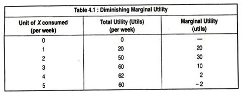
Table 4.1 gives some hypothetical figures showing the total and marginal utility derived by a consumer from consumption of product X. When the individual consumes one unit, he derives 20 utils of satisfaction. When he consumes two units in the week, his total utility rises to 50 utils and so on.

The figures for marginal utility eventually decline as each successive units are consumed. This is called the Law of Diminishing Marginal Utility.

If we assume that consumers are utility-maximisers, i.e., they wish to obtain as much utility as they can, subject to no other constraints, the consumer in Table 4.1 would consume 4 units of X where total utility is greatest.

However, two complicating factors need to be considered:

(a) The consumer’s income is limited,

(b) The consumer must distribute expenditure between many different commodities.

Assume that the consumer has a choice between two products X and Y. If X and Y both cost £1 each, and the consumer has £1 to spend, then the commodity which yields the greatest utility will be bought.

If we were to apply this principle to each successive unit of the consumer’s spending, then we could conclude that utility will be maximised when income has been allocated in such a way that the utility derived from one extra pound’s worth of X is equal to the utility derived from the consumption of one extra pound’s worth of Y.

If this condition is not satisfied then the consumer could obviously increase the total utility by switching expenditure from X to Y, or vice versa.

The extra satisfaction derived from the consumption of one more unit of X is its marginal utility which we can write as MU_X and that of Y as MU_Y, etc. We must consider the relative price of X and Y which we can write as P_X and P_Y.

We can see that the utility-maximising condition is fulfilled when:

MU_X/P_X = MU_Y/P_Y

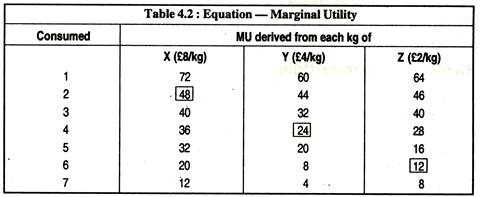
Any number of commodities may then be added to the equation. Table 4.2 gives marginal utility figures for a consumer who wants to distribute expenditure of £44.00 between three commodities, X, Y and Z:

In order to maximise utility, the consumer must distribute available income so that MU_X/P_X = MU_YP_Y = MU_Z P_Z.

From the table, we can see that this yields a selection where the consumer buys 2 kg of X 4 kg of K and 6 kg of Z.

Hence:.48/8 = 24/4 = 12/2 = 6.

This gives the consumer greatest total utility by spending all the £44.00. It is impossible to distribute it in any other way to increase his utility.

Demand and Marginal Utility # 4. Demand Curve:

The marginal utility approach gives us a rationalisation of the demand curve. We start from a condition of equilibrium, where MU_X/P_X = MU_Y/P_Y the price of X falls relative to Y We now have a condition where the utility from the last pound spent on X will be greater than the utility from the last pound spent on Y. This can be written as MU_X /P_X > MU_Y / P_Y.

The consumer can now increase his total utility by consuming more of X This will have the effect of decreasing the marginal utility of X and he will continue increasing his expenditure on X until the equality is restored.

We now have the result we have been seeking : that a fall in the price of a good will, ceteris paribus, give rise to an increase in a consumer’s demand for it — that is to say, the demand curve slopes downwards from left to right. Suppose, initially we have MU_X = 20 utils, MU_Y = 25 utils, P_X = 4 and P_Y = 5 so that the condition of utility is satisfied 20/4 = 25/5 or MU_X /P_X = MU_Y /P_Y.

Now, let the price of X fall to £2 with the consumption unchanged, MU per £ of X rises to 10 utils > MU per £ of Y. How will the consumer respond to this? By spending an extra pound on good X, he derives 10 utils of utility; by spending an extra pound on Y, he derives only 5 utils. Thus, he will buy more of X, reducing MU_X until the MU’s per pound for X and Y are once again equal.

Thus, we have attained the normal demand relationship that, other things being equal, as the price of X falls, more of it is bought, we have, thus, a normal downward-sloping demand curve. The demand curve we have derived is the individual’s demand curve for a product. The market demand curve can then be obtained by aggregating horizontally all the individual demand curves.

This gives us the price (or substitution) effect.

Demand and Marginal Utility # 5. Indifference Curve Analysis:

The marginal utility approach is subject to the major criticism that we have never found a satisfactory way of quantifying utility. In the 1930s, a group of economists came to believe that cardinal measurement of utility was unnecessary.

They argued that demand behaviour could be explained with ordinal number because individuals are able to rank their preferences saying that they would prefer this bundle to that bundle and so on.

Finite measurement of utility becomes unnecessary and it is sufficient simply to know consumers’ preferences Indifference curve analysis can explain this. An indifference curve represents all combinations of baskets that provide the same level of satisfaction to a person.

The theory of consumer behaviour begins with three basic assumptions regarding peoples’ preferences for one basket over another:

The first assumption is that preferences are complete, which means that consumers can compare and rank all baskets.

The second assumption is that preferences are transitive, which means that if a consumer prefers basket A to basket B and prefers B to C, then he also prefers A to C.

The third assumption is that all goods are “good”, so consumers always prefer more of any good to less.

These three assumptions form the basis of consumer theory. They do not explain consumers’ preferences, but they do impose a degree of rationality and reasonableness on them. We add another one to these three assumptions, that, indifference curve is convex to the origin.

Demand and Marginal Utility # 6. Indifference Curves:

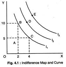
In order to explain indifference curves, we will make simplifying assumption that the consumer only buys two goods or two baskets of goods — X and Y. The consumer’s preference for X and Y are represented by the indifference map in Fig. 4.1, where l_1, I₂, and I₃ are three indifference curves.

An indifference map is a set of indifference curves that describes a person’s preferences. Any combinations on indifference curve 3, such as E, is preferred to any market basket on curve 2, D, which, in turn, is preferred to any basket on 1, such as B or C. An indifference curve joins together all the different combinations of two baskets of goods which yield the same utility to the consumer.

In Fig. 4.1, the vertical axis measures the quantity of good Y and the horizontal axis measures the quantity of good X. Thus, every point on the graph represents some combinations of X and Y. A point very close to the origin, like A, represents very small quantities of X and Y; points further away from the origin represent bigger quantities.

Since points B and C are on the same indifference curve, the consumer is said to be indifferent between them, both combinations yield the same utility to him. Combination D is on a higher indifference curve than B or C. Thus, D is preferred to B and C. Similarly, E is preferred to A, B, C and D.

We assume that the consumer can rank his preference over the entire field of choice. This means that the consumer must be able to consider any two possible combinations of X and Y and say either that he prefers one to the other, or he is indifferent between them.

We assume further that our consumer is rational and must satisfy the following conditions:

(a) He must be able to raise his preferences over the entire field of choice facing him.

(b) His behaviour must be transitive if he prefers combination A to B, and combination B to C, then he must also prefer A to C.

(c) He must never have all he wants of all goods — he must always want some more of at least one good.

We must consider several important features of indifference curves.

Demand and Marginal Utility # 7. Indifference Curves Slope Downwards from Left to Right:

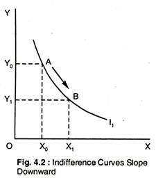
If both X and Y are goods and if the consumer is rational, then we must conclude that if consumers give up some of X, they will want more of Y to remain at the same level of utility. Consider Fig. 4.2. In moving from A to B, as units of Y are given up, more units of X are obtained and the utility derived is unchanged. For this to be true, the indifference curves must slope downwards from left to right.

Demand and Marginal Utility # 8. Indifference Curves are Convex to the Origin:

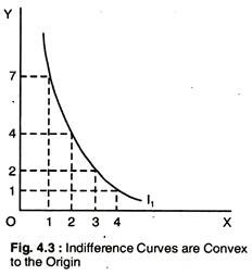
As more and more units of one good, say Y, are given up, it is reasonable to suppose that successively bigger quantities of X must be obtained to compensate the consumer for his loss and leave him at the same level of utility.

In Fig. 4.3, this proposition is considered. Since the slope of an indifference curve is called the marginal rate of substitution (MRS), the proposition is sometimes summed up as the diminishing marginal rate of substitution.

The slope of the indifference curve measures the consumer’s MRS between two goods. In Fig. 4.3, the MRS between Y and X is — ΔY/ΔX, falls from 3 to 2 to 1. When the MRS diminishes along an indifference curve, preferences are convex. The MRS at any point is equal, in absolute value, to the slope of the indifference curve at the point.

Demand and Marginal Utility # 9. Indifference Curves can never Intersect:

This is shown in Fig. 4.4. Since A and C are on the same indifference curve, the consumer must be indifferent between them. Combination B and C are also on the same indifference curve, so the consumer must be indifferent between them as well.

If a consumers is indifferent between A and C, and between B and C, he must (by the rule of transitivity) be indifferent between A and B. This is absurd and illogical because A contains more Y and the same amount of X as B and so must be preferred to it. This kind of absurd result occurs whenever indifference curves intersect. We conclude, thus, that indifference curves can never intersect each other.

Demand and Marginal Utility # 10. Ordinal lersus Cardinal Rankings:

We have shown only 3 indifference curves in Fig. 4.1. The three curves provide an ordinal ranking of baskets of goods. An ordinal ranking places baskets in the order of most preferred to least preferred, but it does not indicate by how much one market basket is preferred to another. For example, we know that consumption of any basket on IC₃, such as E, is preferred to consumption of any basket on IC₂, such as D.

However, the amount by which E is preferred to D is not revealed by the indifference map. By contrast, when economists first studied utility, they assumed that individual preference could easily be measured in terms of basic units and could, therefore, provide a cardinal measurement.

However, we now know that the particular unit of measurement is not important, and an ordinal ranking is sufficient to help us explain how most individual decisions are made.

Demand and Marginal Utility # 11. Budget Lines and Consumer’s Equilibrium:

Indifference curves only tell us about the consumer’s preferences for two goods. They cannot tell us which combinations will be chosen. In addition to the consumer’s preferences, we need to know his budget constraints, i.e., income and the prices of the two goods.

Given these information, and assuming that he will choose the combinations of two goods which will yield him greatest utility, we can find out the combination of X and Y that the consumer will choose. For example, suppose the price of X is £2, the price of Y is £1, and the consumer’s income is £100.

Now we can draw the budget line which shows all the combinations of two goods which can be purchased with a given level of income and the relative prices of the two goods. With £100, we can either consume 100 units of Y and no X or 50 units of X and no Y. This is illustrated in Fig. 4.5(a). It shows the combinations of the two goods that can be purchased with an income of £100.

The slope of the budget line – P_X/P_Y = 2 (100/50) measures the relative price of X in terms of Y— that is, 1/2 units of Y must be given up in order to buy one unit of X.

The slope of the budget line is (P_X/P_Y) where P_X = price of X and P_Y the price of Y or ΔY/ΔX = -1/2 measures the relative cost of X and Y. AF line shows the budget associated with an income of £100, a price of Y, P_Y = £1, and a price of X, P_X = £2. The slope of the budget line is – P_X/P_Y.

Demand and Marginal Utility # 12. Consumer Choice:

Given preferences and budget constraints, we can choose how much of each good to buy. We assume that consumers make this choice to maximise the satisfaction, given budget constraint. Now we draw indifference map on the graph 4.5(b). Assuming that the consumer spends all his income on X and Y, he will choose the combination represented by C.

This is the point where the budget line is tangential with an indifference curve – the indifference curve I₂ is the highest one that can be reached. Point C is called the consumer equilibrium point where he maximises his utility subject to his budget constraint.

At point C, the slope of the indifference curve (MRS) is equal to the slope of the budget line at that point. Thus we can write that, at the consumer equilibrium point, slope of the budget line => P_x/Y_y= MRS.

It may be noted that point B on IC₁, is not the most preferred choice, because a reallocation of income in which more is spent on X and less on clothing (Y) can increase the consumer’s satisfaction In particular, by moving to point C, the consumer spends the same amount but achieves a higher level of satisfaction associated with IC₂, IC₃, will give a still higher level of satisfaction but cannot be reached with the available income.

Thus, C maximises the consumer’s satisfaction.

Demand and Marginal Utility # 13. Perfect Substitute and Perfect Complement:

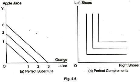
In Fig. 4.6(a) consumer views orange juice and apple juice are perfect substitutes; consumer is indifferent between a glass of one and the other. The IC_S with perfect substitute have a constant slope. In Fig. 4. 4.6(b) consumer views left shoes and right shoes as perfect complements. An additional left shoe gives consumer no extra satisfaction unless consumer also obtains the matching right shoe.

Demand and Marginal Utility # 14. Effect of Income Change:

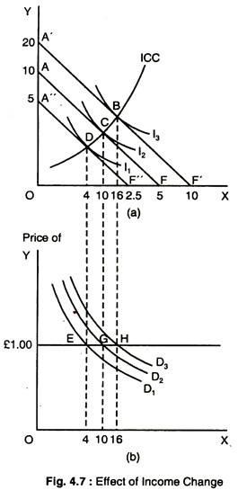
If the consumer’s income increases, his budget line will shift upwards remaining parallel to the original one. Similarly, if his income falls, his budget line will shift downwards remaining parallel. Suppose that the consumer’s income rises from £100 to £200.

The new budget line A’F’, together with the original one AF, is shown in Fig. 4.7. Now suppose that his income falls to £50 and the new budget line A”F” is also shown in Fig. 4.7.

With an income of £200 the consumer equilibrium point is shown as point B in Fig. 4.7. With an income of only £5o’ the consumers equilibrium point is D. The important result to remember is that when income changes, the budget line shifts but remains parallel. DCB is called the income-consumption curve. It shows what happens to the consumer’s demand for the two goods as his income changes.

Demand and Marginal Utility # 15. Effect of Price Change:

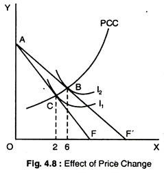
We now examine the effect of a price change. Suppose the price of X falls, ceteris paribus. The new budget line AF’ is drawn together with the original one AF in Fig. 4.8. Income is still £100, the price of Y is £1 as before and the price of X has fallen to £1. When the price of one of the goods falls, the budget line does not shift, but this pivots and so does not remain parallel to the original one.

It becomes less steep reflecting the fall in the relative price of X. The effect of the price fall on the consumer equilibrium point is shown in Fig. 4.8, it moves from point C to point B. The line CB is called the price- consumption curve. The fall in the price of X causes the consumer’s demand for it to increase from 2 to 6.

There are two possible reasons for this:

(a) As the price of X falls, it becomes relatively cheaper and Y becomes relatively more expensive. The consumer is, thus, induced to substitute X for Y. This is called the substitution-effect of the price change.

(b) As the price of X falls, the consumer is now better-off — he experiences an increase in his real income. This may allow him to buy more of X and more of Y. This is called the income effect of the price change.

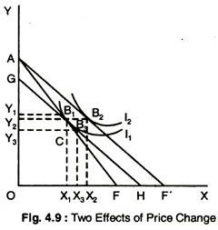
It is possible to identify these two effects graphically and this is done in Fig. 4.9. The first step is to eliminate the income effect: to do this, we assume that, accompanying to fall in the price of X, there is a compensating variation in income which leaves the consumer at the same level of utility as before the price change.

In Fig. 4.9, the original budget line is labelled AF whilst the new budget line after the price change is labelled AF’. To make the compensating variation in income, we draw a new budget line parallel to AF’ until it becomes tangential to the original indifference curve I₁.

The new budget line is GH and the movement of consumer’s equilibrium point from B₁ to B₃ is the substituted effect — the consumer is no better-off, but has substituted X₁ X₃ of X for Y₁Y₃ of Y because of the change in relative prices. The movement from B₃ to B₂ is due to income effect — the consumer buys X₃X₂ of X and Y₃Y₂ of Y because of his increase in real income.

Demand and Marginal Utility # 16. Normal, Inferior and Giffen Goods and IC:

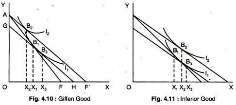
The substitution effect always acts in such a way that when the relative price of a good falls (real income remaining constant), more of it is purchased. The income effect can work either way — when the consumer’s real income rises, he may buy more or less of X. If he buys more, it is a normal good: this is shown in Fig. 4.9, when both X and Y are normal goods.

If he buys less, the good is an inferior good this is shown in Fig. 4.11 — where the movement from to B₂ is the negative income effect. If he buys less, and the income effect is actually bigger than the substitution effect so that the overall effect of the price fall is decreased in consumption, then the good is a Giffen good: this is shown in Fig. 4.10 — where the negative income effect (B₃ to B₂) is bigger than the substitution effect (B₁ to B₃).

Demand and Marginal Utility # 17. Derivation off the Demand Curve for a Normal Good:

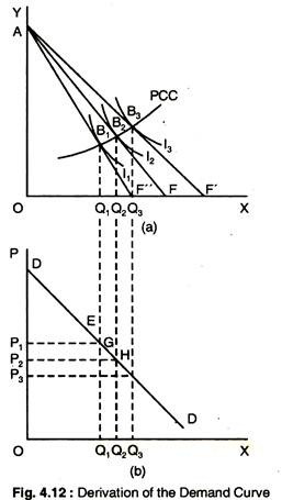
From the previous analysis we can derive a consumer’s demand curve. The price- consumption curve in Fig. 4.8 shows the different points of ‘consumer’s equilibrium’ as the price of X is varied, ceteris paribus. It gives sufficient information to draw consumer’s demand curve from indifference curve. ”

This is done is Fig. 4.12 where X is a normal good: as the price of X is reduced from OP₁ to OP₂ to OP₃, the quantity of X demanded expands from OQ₁ to OQ₂ to OQ₃. The resulting demand curve is downward-sloping from left to right.

We have completed a full circle. Having started by considering an individual consumer’s demand curve in isolation, we have looked at the concept of utility and the theory of consumer behaviour which underlies demand.

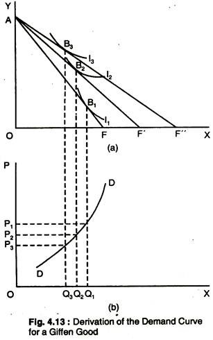
Moreover, we have also seen that by making certain assumptions about the consumer’s preferences and assuming ceteris paribus, we can derive a demand curve which slopes downwards from left to right. Under certain exceptional circumstances, a demand curve which slopes upwards from left to right is drawn in Fig. 4.13.

Demand and Marginal Utility # 18. Derivation of the Demand Curve for a Giffen Good:

Demand and Marginal Utility # 19. Consumer’s Surplus:

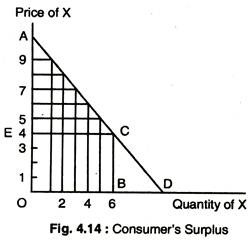
We now consider individual demand curve for good X as shown in Fig. 4.14 and suppose that the prevailing market price is £4. It is clear from Fig. 4.14 that the individual will buy 6 units of the good per week, paying £24 and from the foregoing analysis we know that he will maximise his utility by these purchases.

Consider also that the first unit of X, that he buys yields him so much utility that he would have been prepared to pay as much as £9 for it.

Similarly, he would have been prepared to pay £8 for the second unit, £7 for the third unit and so on. Since a single price of £4 prevails iii the market, he has only had to pay £24 for the six units (area OBCE), instead of £39 (area OACB). The difference (£39 – £24 =) £15 can be thought of as the consumer’s surplus and is represented by the area under the demand curve and above the price line ECA.

Demand and Marginal Utility # 20. Revealed Preference Theory:

This theory is based on the assumption that a consumer will actually choose to consume the collection of goods that he prefers.

Samuelson used this proposition to derive a consumer’s downward-sloping demand curve in such a way that required neither the subjectivity of the utility concept used in both the ordinal and cardinal utility approaches, nor the assumption of diminishing marginal utility of the cardinalist approach. All that was required was that the consumer behaved consistently.

The ‘revealed preference’ theory can demonstrate that the consumer’s demand curve for a good will be downward-sloping from left to right so long as the consumer is observed to increase his purchase of the good when his income increases or price decreases.

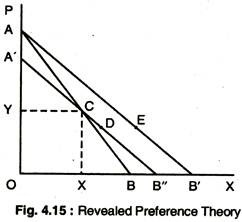
Suppose that the line AB in Fig. 4.15 is a consumer’s budget line and the point C is the combination of X and Y that the consumer reveals preferred compared to other combinations attainable in the triangle AOB.

If the price of X falls, the budget line will shift to AB’. The income effect of this price change can be eliminated by shifting the budget line to A ‘B” parallel to AB. Having revealed that the consumer preferred point C to any other points in the triangle AOB, he will not now choose any points along the section A’C. He must, therefore, choose a point along the line CB”, say point D.

The movement from C to D is the substitution effect of the price fall and thus, consumer purchases more of X following the price fall. If the income effect also causes him to buy more of X, then he must move to point E on the budget line AB’ to the right of point D.

Since the fall in the price of X has induced the consumer to buy more ceteris paribus, we conclude that the consumer’s demand curve slopes downwards from left to right.

It is important to notice that, to arrive at this conclusion, no mention of the abstract concept of utility was made. Thus, the revealed preference theory can be described as a more objective approach to the theory of consumer behaviour.

However, some subjective element is still implicit when consumers reveal their preferences for goods. The theory places « a great emphasis upon rationality which may not be observed in reality.

A possible reason for this is that consumers are often swayed by differences within a product. For example, the minor differences in brands of washing powder which may seem trivial to the logical economists may be important to the consumer, who is willing to pay for them. Those who work on advertising are well aware that it is often the emotional content of a product which is more important than the rational.

This does not necessarily contradict our analysis — as Lancaster argues it is the characteristics or attributes of goods which yield satisfaction to the consumer, rather than the goods themselves.

According to this approach we should analyse a consumer’s choice between different brands on the assumption that the consumer is attempting to maximise the utility he derives from the characteristics possessed by the goods, rather than the goods themselves.

We have examined the various approaches to the analysis of consumer behaviour, and looked more closely into the proposition that a fall in the price of a normal good will cause an increase in the quantity of that good demanded by an individual consumer.

Demand and Marginal Utility # 21. Engel Curves:

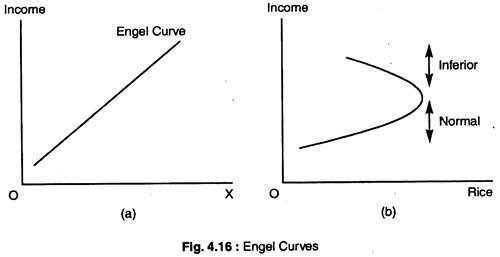
Income-consumption curves can be used to construct Engel curves, which relate the quantity of a good consumed to income. Fig. 4.16 shows how Engel curves can be constructed for two different goods. Fig. 4.16(a) shows an upward-sloping Engel curve, which is derived directly from Fig. 4.7(a).

In both figures, as income increase, the consumption of X also increases. The upward-sloping Engel curve applies to all normal goods. Figure 4.16(b) shows the Engel curve for rice. We see that rice consumption increases initially as income increases. As income increases further, consumption falls. The portion of the Engel curve that is downward-sloping is the income range in which rice is an inferior good.

Demand and Marginal Utility # 22. Market Demand:

So far we have discussed the demand curve for an individual consumer. But here we show how market demand curves can be derived as the sum of the individual demand curves of all consumers in a particular market.

From Individual to Market Demand:

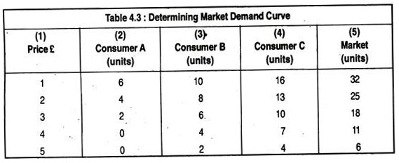
For simplicity, let us assume that there are only three consumers for coffee in the market. Table 4.3 presents several points on each of these consumers’ demand curves. The market demand, column (5), is found by adding columns (2), (3) and (4) to determine the total quantity demanded at each price. For example, when the price is £3, the total quantity demanded is 2 + 6+10=18.

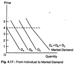
Fig. 4.17 shows these three consumers’ demand curves for coffee (labelled D_A, D_B and D_C). In the figure, the market demand curve is the horizontal summation of the demands of each of the consumers. We sum horizontally to find the total amount that the three consumers will demand at any given price.

For example, when the price is £4, the quantity demanded by the market (11 units) is the sum of the quantity demanded by A (no units), by B (4 units) and by C (7 units). Because all the individual demand curves slope downward, the market demand curve will also slope downward.

However, the market demand curve need not be a straight line, even though each of the individual demand curves is. In Fig. 4.17, for example, the market demand curve is kinked as one consumer makes no consumption at prices.

Two points should be noted here. First, the market demand curve will shift to the right as more consumers enter the market. Second, factors that influence the demands for many consumers will also affect the market demand.

For example, suppose that most consumers in a particular market have more income, and, as a result, increase their demand for coffee. Since each consumer’s demand curve shifts to the right, so will the market demand curve.

The aggregation of individual demands into a market demand is not just a theoretical exercise, but also important in practice.

For example, we can obtain information about the demand for home computers by adding independently about the demands of:

(i) Households with children,

(ii) Households without children, and

(iii) Single individuals.

Demand and Marginal Utility # 23. Some Useful Examples:

Example 1: Decision-making of a Local Public Official:

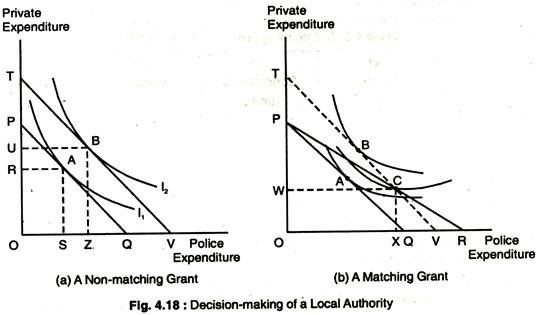
Grant programmes from the central government to local governments; suppose that a public official is in charge of the police budget, which is paid for by local taxes. His preferences reflect what he believes should be allocated for police spending and what he feels citizens would prefer to have available for private consumption.

Before the introduction of the grant programmes, the city’s budget line is PQ, as in Fig. 4.18. This budget line represents the total amount of resources available for public police spending (on the horizontal axis) and private spending (on the vertical axis). The preference-maximising point A on indifference curve I₁ shows that OR is spent on private spending and OS on police expenditures. Since public expenditures are paid for by local taxes, these private expenditures represent spending after local taxes have been paid.

There are two types of grants a non-matching grant and matching grants. Fig. 4.18(a) — A Non-matching Grant: A non-matching grant from the central government to a local government acts just like an increase in income in the traditional consumer analysis.

The local government official moves from A to B, thereby allocating a portion of the grant to public expenditures and a portion to lower taxes and, therefore, to increase private expenditures. An unconditional grant shifts the community budget line outward from PQ to TV, where PT = QV, as in Fig. 4.18(a). The response to this grant is to move to a higher indifference curve by selecting point B, with more of both goods.

A matching grant acts like a price decrease in the traditional consumer analysis. For example, the central government might offer to pay £1 for every £2 that the local government raises to pay for police.

As a result, a matching grant lowers the relative cost of the publicly provided goods. In Fig. 4.18(b), the matching grant relates the budget line outward from PQ to PR. If no local money is spent on police, the budget line remains unchanged. However, if they decide to spend money on the public sector, the budget increases.

In response to the matching grant, the official chooses point C rather than A which involves an increase in both police and private expenditures. At C, OW is allocated to private expenditures and OX on police expenditures. However, the spending effects of the matching grant are different from those of a non-matching grant.

The diagram shows that the matching grant leads to greater police spending than does the non-matching grant when the two grant programmes involve identical government expenditure.

Demand and Marginal Utility # 24. A Corner Solution:

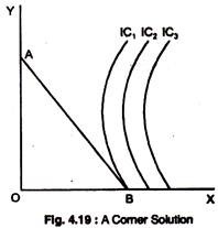
The indifference curve analysis can be used to show conditions under which consumers choose not to consume a particular good. In Fig. 4.19, faced with budget line AB, a consumer chooses to purchase only X and no Y.

This is called a corner solution because when one of the goods is not consumed, the consumption bundle appears at the corner of the graph that describes the consumer’s budget line. At B, which is the point of maximum satisfaction, the MRS X for Y is greater than the slope of the budget line.

When a corner solution arises, the consumer’s MRS is greater than the price ratio for all levels of consumption. The consumer maximises satisfaction by consuming only one of the two goods. Given budget line AB, the highest level of satisfaction is achieved at B on indifference curve 1, and only X is consumed.

Optimal Choice with Perfect Substitutes:

If the goods are perfect substitutes, the optimal choice will usually be on the boundary.

Optimal Choice with Concave Preferences:

The optimal choice is the boundary point.

Example 2: A College Trust Fund:

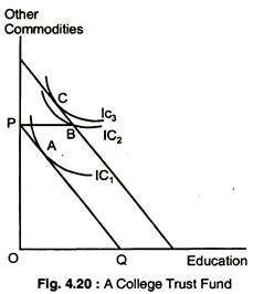
Peter’s parents have provided a trust fund for his college education. The mist fund is a welcome gift to Peter but perhaps not as welcome as an unrestricted trust would be. In Fig. 4.20, pounds per year spent on Peter’s education are shown on the horizontal axis, and pounds spent on other forms of Peter’s consumption are shown on the vertical axis.

The budget line that Peter faces before the trust fund being awarded is given by PQ. The trust fund expands the budget line outward so long as the full amount, PB, is spent on education. By accepting the trust fund and going to college, Peter increases his satisfaction, moving from A on IC₁, to B on IC₂.

It may be noted that B represents a corner solution because Peter’s MRS of other consumption for education is lower than the relative price of other consumption. Peter would prefer to spend a portion of the trust fund on other goods as well as education. Without the restriction on trust fund, he would move to point C on IC₃, decreasing his spending on education but increasing his spending on other goods. For the trust recipient, a restricted trust would be less beneficial than an unrestricted trust. Restricted trusts are popular because they enable parents to control their children’s expenditures.

Demand and Marginal Utility # 25. Indifference Curve for Bads:

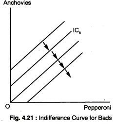
A bad is a commodity that the consumer does not like. For example, suppose that commodities in question are now pepperoni and anchovies — and the consumer likes pepperoni and dislikes anchovies. How could we represent these preferences using indifference curves?

Suppose our consumer picks a bundle (x₁, x₂) consisting of some pepperoni and some anchovies. If we give the consumer more anchovies, what do we how to do with the pepperoni to keep him on the same indifference curve? Definitely, we have to give him some extra pepperoni to compensate him. Thus, this consumer must have IC_S that slope up and to the right as in Fig. 4.21 below.

The direction of increasing preference is down and to the right — that is, towards the direction of decreased anchovy and increased pepperoni, just as the arrows in the diagram illustrate.

Demand and Marginal Utility # 26. Neutrals and Bads:

In the case of a neutral good, the consumer spends all of her money on the good she likes and does not purchase any of the neutral good. The same thing happens if one commodity is a bad. If X₁ is a good and X₂, is a bad, then the demand functions will be X₁ =  m/p₁; X₂ = 0 as in Fig. 4.21.

Demand and Marginal Utility # 27. Neutrals:

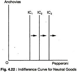
A good is a neutral good if the consumer does not care about it one way or the other. Suppose the consumer is neutral about anchovies. In this case, indifference curves will be vertical lines as given in Fig. 4.22.