
In this article we will discuss about the marginal productivity theory that discusses the demand for a variable factor of production.
Introduction Marginal Productivity Theory (MPT):
The leading exponents of the marginal productivity theory (MPT) are the neoclassical economists J. B. Clark (1847-1938), P. H. Wicksteed (1844-1927) and J. G. Knut Wicksell (1851- 1926). This theory especially discusses the demand for a variable factor of production, and it does not throw any light at all on the supply of the inputs. That is why MPT is not considered as a complete theory of factor price determination.
The main contention of the MPT is that a variable input, say, labour, would get a price equal to its marginal product (MP). The increment in the total product of a firm that would be realised when an additional unit or the marginal unit of labour (the variable factor) is used, is known as the marginal physical product of labour (MPPL or MPL).
The Assumptions of the MPT:
The MPT is based on certain assumptions:
ADVERTISEMENTS:
(i) The firm uses only one variable input, say, labour, along with some other fixed inputs, and there is no problem in using labour in variable quantities with the fixed inputs.
(ii) There exists perfect competition in both the factor (labour) and the product markets. That is, in the labour market, a large number of buyers and sellers are buying and selling a homogeneous labour input, and, in the product market, a large number of buyers and sellers are buying and selling a homogeneous product.
(iii) The quantity of labour (L) used by a firm is a continuous variable, i.e., it is possible to measure L in infinitesimally small units.
(iv) The law of variable proportions (LVP) operates in the field of labour employment, i.e., as the quantity of labour used (L) increases, MPPL increases in the initial stages, and, after a certain point, as L increases, MPPL diminishes.
ADVERTISEMENTS:
(v) The goal of the firm is to obtain the maximum amount of profit, i.e., the firm would use the quantity of labour at which its profit would be maximum.
Measuring the Marginal Product:
Estimates of the marginal product (MP) of a variable input (labour) may be expressed in three different forms. These are:
(i) Marginal Physical Product of Labour (MPPL or, Simply, MPL):
The increment in the total physical product of labour (TPPL or TPL) of the firm that is obtained when an additional (or the marginal) unit of labour has been used is known as the marginal physical product of labour (MPPL or MPL).
ADVERTISEMENTS:
According to this definition, we shall obtain the MPPL when the quantity of labour used is n units if we subtract TPPL at (n – 1) units of labour from the TPPL at n units of labour. We may write, therefore,
[MPPL] at L = n units = [TPPL] at L = n units – [TPPL] at L = n- 1 units (15.1)
(ii) Value of Marginal Physical Product of Labour (VMPPL):
If we multiply MPPL by the price of the product (p), we obtain the value of marginal physical product of labour (VMPPL or VMPL).
Therefore, we may write:
VMPPL = MPPL x p (15.2)
Estimates of VMPPL are obtained in units of money.
(iii) Marginal Revenue Product of Labour (MRPL):
ADVERTISEMENTS:
First, let us note that the revenue of the firm obtained by selling the product of the firm that is produced by a particular quantity of labour, say, L = n units, is called the total revenue product of labour (TRPL) at L = n units.
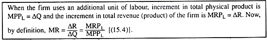
Now, the marginal revenue product of labour (MRPL) is defined as the increment in TRPL obtained when an additional (or the marginal) unit of labour has been used.
Therefore, We may Write:
[MRPL]L = n units = [TRPL]L = n units _ [TRPL]L = n- 1 units (15.3)
ADVERTISEMENTS:
Obviously, the estimates of MRPL are also obtained in terms of money.
The VMPPL and the MRPL Curves:
In Fig. 15.1(a), the VMPPL = MRPL curve is the VMPPL curve and, at the same time, it is the MRPL curve. These two curves would be obtained as the same curve, because the assumption of perfect competition in the product market would give us VMPPL = MRPL at any L.
This we may prove in the following way:
According to the definitions, at any L and at the corresponding quantity of output (Q) produced and sold, we obtain
ADVERTISEMENTS:
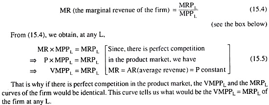
ADVERTISEMENTS:
In Fig. 15.1(a), the shape of the VMPPL = MRPL curve has been like an inverted-U, because, the MPPL curve is like an inverted-U owing to the law of variable proportions and VMPPL is nothing but MPPL x P where P is a constant.
The ARPL Curve:
In Fig. 15.1(a), the average curve associated with the marginal MRPL curve is the Average Revenue Product of Labour (ARPL) curve, From this ARPL curve, we may obtain TRP ARPL = TRPL/L at any L. The shape of the ARPL curve is also like an inverted-U owing to such a shape of the MRPL curve. The MRPL curve, while sloping downwards, would intersect the ARP, curve at its maximum point.
ADVERTISEMENTS:
These features are obtained from the average-marginal relation. The ARPL curve has been inserted in Fig. 15.1, because, this curve would help us to know the cut-off rate of wage, beyond which, if W rises, the firm would shut down its production.

The AEL and MEL Curves:
In MPT, it has been assumed that there is perfect competition also in the labour (factor) market.
Because of this assumption, the firm may buy any quantity of labour it requires at a constant rate of wage (W) which has been determined in the market, and that is why we obtain at any L:
W = AEL = MEL = constant (15.6)
where W = the rate of wage = constant
ADVERTISEMENTS:
AEL = average expense for labour = W
and MEL = marginal expense for labour
From (15.6), we obtain that the AEL = MEL curve of the firm is a horizontal straight line at the level of W. In Fig. 15.1, firm’s AEL = MEL curve is AE(1)L = ME(1)L, when W = W1.
Conditions for the Equilibrium Quantity of Labour to be Purchased and used by the Firm:
In MPT, it is assumed that the goal of the firm is to maximise profit. Therefore, at the equilibrium point, the firm would buy such a quantity of labour that would enable it to maximise the level of profit.
Now, by definition, the profit (π) of the firm, at any L, is:
ADVERTISEMENTS:
π = TRPL-TEL-TFC (15.7)
where TRPL = total revenue product of labour,
TEL = total expense for labour = total variable cost of the firm (TVC) (since labour is the only variable input)
TFC = total fixed cost, i.e., the total cost of the firm for the fixed inputs = constant. Since TFC = constant in (15.7), 71 would be maximum when TRPL – TEL is maximum.
Let us suppose:
πL = TRPL-TEL (15.8)
=>π = πL-TFC [from (15.7)] (15.9)
Now, since TRPL and TEL are both functions of L in (15.8), πL is also a function of L. Therefore, πL has to be maximised w.r.t. L.
The first order condition (FOC), or the necessary condition, for the maximum πL, and, therefore, for maximum π, is:
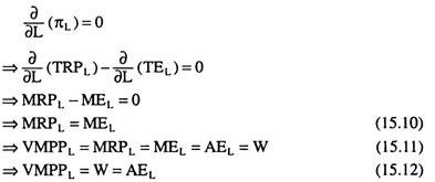
The first order conditions (15.10) and (15.12) give us that the profit-maximising quantity of labour for the firm would be obtained at the point of intersection between its MRPL and MEL curves or between its VMPPL and AEL curves.
These two points would be the same since VMPPL = MRPL, and AEL= MEL = W. Again, (15.12) also gives us that the firm would buy that quantity of labour at which the VMPPL and the rate of wage would be equal. It may be remembered here that the VMPPL = W, i.e., the labour would get a rate of wage equal to the value of its marginal physical product, is the main contention of the MPT.
Now, the second order condition (SOC) or the sufficient condition for the maximisation of πL (and also of π) is:
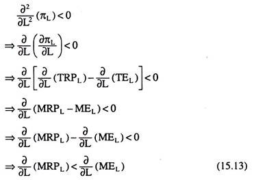
What we obtain from (15.13) is that the slope of the MRPL (= VMPPL) curve should be less than the slope of the MEL curve at the point of maximum profit—this is the sufficient condition.
Since the MEL curve here is a horizontal straight line (slope = 0), FOC and SOC, i.e., (15.10) and (15.13) imply that, at the point of maximum profit, i.e., at the point of intersection between the MRPL and MEL curves, the slope of the MRPL curve would be negative, i.e., this curve would be sloping downward towards right. That is,
∂/∂L (MRPL) <0 (15.14)
Economic Interpretation of the First Order and Second Order Conditions for Maximum Profit:
We may give the economic interpretation of the FOC and the SOC, (15.10) and (15.13), in the following way:
Let us suppose that, in Fig. 15.1, the rate of wage (W) that has been determined in the labour market is W = W1. Now, at any L, for example, at L = L3, the profit of the firm obtained from the marginal unit of labour (i.e., the marginal profit) would be positive if we have MRPL > MEL = AEL = W = constant.
For here the revenue product (i.e., revenue) obtained from the use of the marginal unit of labour is greater than the expense for this labour unit.
Now, if the profit from the marginal labour unit is positive, then the profit-maximising firm would be increasing the quantity of labour (L) to be used by it. And as L increases, the MRPL may rise and then fall (because of its shape of an inverted-U), and eventually it would fall to the level of MEL = constant, as we have obtained at the point E, in Fig. 15.1(a).
The firm would not increase L beyond this point (E,) because then its MRPL would fall below the level of MEL, i.e., it would have MRPL < MEL, and in that case, the firm would suffer loss on the marginal unit (its marginal profit will be negative). At the point E1, the FOC and SOC, (15.10) and (15.13), have been satisfied, since E1 is the point of intersection of the MRPL and MEL curves and, at E1, the MRPL curve is negatively sloped.
We have to remember here that at the MRPL = MEL point like F1, the firm’s profit would not be maximum, because if L increases beyond this point, the firm would have MRPL > MEL, and a positive marginal profit, which implies that it still has a scope of increasing its total profit by increasing L.
So, at the point like F1, profit cannot be maximum. The firm would be increasing L in its quest for maximum profit till its MRPL comes down to the level of MEL at the point E1. It may be observed that at the MRPL = MEL point F1, the FOC has been satisfied but the SOC has not been satisfied because at F1, the MRPL curve is upward sloping—it is not downward sloping as required by the SOC.
A Third Condition—πL ≥ 0:
We have obtained above the FOC and SOC, (15.10) and (15.13), for maximisation of πL (and of π). Mathematically, we would have the maximum πL (and n) if these two conditions are satisfied. However, calculus does not ensure that the maximum πL would not be negative. On the contrary, at some values of W, the maximum πL may very well be negative.
Let us see its implications. We have πL < 0 ⇒ TRPL < TEL [eq. (15.8)]. That is, if πL < 0, then the total revenue product of labour (which is total revenue as a function of L) would be less than the total expense for labour, which means the firm would have to borrow to pay the (TEL – TRPL) portion of its labour expenses, and over and above this, the firm would have to borrow to meet its total fixed cost (TFC) obligations.
Therefore, in such an eventuality (πL < 0), the total amount of loss that the firm would have to bear would be TEL – TRPL + TFC. Now, if the firm shuts down its production in this case, then the amount of labour employment (L) would come down to zero (L = 0) and the firm would not have to borrow anything to pay for its labour cost (we would have TRPL = 0, TEL = 0 and πL = 0).
In this case, the firm’s loss would be equal to its TFC only. This is the minimum amount of loss that the firm would have to bear under the circumstances. That is, what we have obtained is that, if πL < 0, then the firm’s labour employment (and output) would have to be made equal to zero. Only then its loss would be minimised (= TFC) and (negative) profit maximised (= – TFC).
On the other hand, if the firm has kl > 0, then there may be two different possibilities. First, the firm may have πL > TFC > 0. In that case, its k (= πL – TFC) may be positive (k > 0) [eq. (15.9)] and the firm would certainly continue its output production. In the second case, the firm may have 0 < πL < TFC.
In this case, the firm’s K would be negative (π < 0); but it would employ labour and continue its production. For here, the firm would be able to pay for a portion of its TFC with the help of its positive πL, i.e., with the positive amount of (TRPL – TEL).
The firm’s loss in this case would amount to TFC – πL. But the loss would increase and become equal to TFC if the firm discontinues production. In other words, in this case, the firm will continue its operations, for, by doing this, it would be able to minimise the loss or maximise (negative) profit.
Lastly, if the firm has πL = 0 ⇒ TRPL = TEL [eqn. (15.8)], then it would have π < 0, being equal to – TFC, i.e., it would be a losing concern. Here if the firm shuts down, then its loss would be equal to TFC. On the other hand, if it continues, then also its loss would be equal to TFC, for now all its TRPL would have to be used to pay for the labour expenses (TRPL = TEL).
Therefore, if πL = 0, the firm would be indifferent between continuing and discontinuing the production of its output, because, in both cases, it would suffer the same amount of loss.
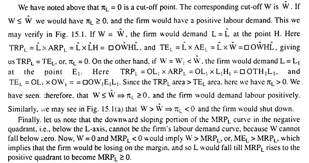
However, since the loss to be suffered when production will continue is not more than that when production will discontinue, we may assume that the firm will prefer continuing with its production when πL = 0. Or, we may put the same thing in a slightly different way. πL = 0 is a cut-off point. If πL ≥ 0, the firm will continue production and L will be positive; if πL < 0, it will shut down its operations and L will be zero.
Therefore, along with the FOC and SOC, (15.10) and (15.13), we get a third condition for the firm’s profit-maximising or loss-minimising labour employment, which is
πL ≥ 0 => π ≥ TFC [eq. (15.9)] (15.15)
Relevance of the ARPL Curve to the Labour Demand Curve of the Firm:
Condition (15.15) gives us:
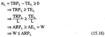
Therefore, condition (15.15) reduces to condition (15.16). This gives us that the firm’s demand for labour will be positive if the rate of wage (W) is less than or equal to labor’s average revenue product.
Now, conditions (15.10), (15.14) and (15.16) imply that the firm’s labour demand curve would be that segment of the downward sloping portion of its MRPL = VMPPL curve that starts from the maximum point of the ARPL curve and lies below it.
Therefore, in Fig. 15.1(a), the segment HE1E2. . . of the MRPL curve would be the firm’s labour demand curve. Conditions (15.10), (15.14) and (15.16) also imply that the firm would demand a positive quantity of labour and continue to produce its output, if the rate of wage lies between 0 and W, both ends inclusive, i.e., if 0 ≤ W ≤ ŵ. That is, this range of W corresponds to the whole length of the labour demand curve HE1E2 . .. . En.
Let us explain:
We may conclude, therefore, that an analysis of the factor demand side of the MPT gives us that the firm’s demand curve for the variable factor, labour, under perfect competition in the product market would be downward sloping to the right, giving us an inverse relation between W and L (labour demand).
It would be the segment of the downward sloping portion of the MRPL curve that starts on and from the maximum point of the ARPL curve and stretches up to the L-axis. Actually, the firm’s labour demand curve is obtained in the second stage of production which is considered to be the efficient stage.
Equality between W and VMPPL:
We have seen in the above analysis that owing to the assumptions of the MPT (especially, assumptions (iii), (v) and (vi), the firm would demand at any particular price (W) that quantity of the variable factor (here labour) at which the MRPL = VMPPL would be equal to W.
For example, in Fig. 15.1, when W = W1 and W = W2, the firm’s demand for labour would be L = L1 and L = L2, respectively. Since W would be equal to VMPPL at any (W, L) combination, labour would always obtain a price that would be equal to the value of its marginal physical product. The main proposition of the MPT is thus established.
Complete and Currently Accepted Version of Marginal Productivity Theory (MPT):
What is known as the neoclassical version of the marginal productivity theory. This theory is so named because it has shown that the input demand is based on the value of the marginal product of the input.
But as a theory of the determination of the input prices based on competition, this theory is considered to be incomplete because it has not analysed the supply side of an input and, therefore, it has not attempted at input price determination through the process of demand-supply interaction.
But we may easily do this job and give the MPT a complete shape. Of course, as we have already noted, inputs vary considerably in respect of the nature of their supply.
Let us first complete the demand side. The MPT has given us the labour demand curve of a firm. We may now have the aggregate demand curve for some homogeneous labour service by taking the horizontal summation of the individual firms’ demand curves. Since the individual curves are downward sloping, the aggregate curve will also be downward sloping like the curve DL in Fig. 15.1(b).
Now, on the supply side let us suppose, for the time being, that the aggregate supply curve of labour, like most other supply curves, will be sloping upwards towards right like the curve SL in Fig. 15.1(b). In the perfectly competitive labour market, the equilibrium rate of wage would be determined in the process of interaction between demand for labour and supply of labour.
In Fig. 15.1, this rate wage is W*. It has been obtained at the point of intersection, G, between the DL and SL curves. At this rate of wage, demand for labour (DL) has been equal to supply of labour (SL) both being equal to N*, and the market is in equilibrium. This equilibrium is a stable equilibrium.
For if W > W*, DL would be less than SL, and there would be an excess supply in the labour market. In this case, the workers would be willing to accept a lower W to be able to sell their (excess) labour, and W would be coming down till it becomes equal to W*.
On the other hand, if W < W*, there would be an excess demand for labour in the market. Now the firms would be willing to offer a higher W to obtain their required labour quantities. As a result, W would be increasing and excess demand falling, till W becomes equal to W*.
At W = W*, there would be neither any excess demand nor any excess supply of labour in the market, and none of the buyers and sellers of labour would remain dissatisfied. Therefore, now the market would be in equilibrium.
In the perfectly competitive labour market, the buyers of labour, or the firms, have to accept the rate of wage (here W*) that has been determined in the market and they would decide what quantity of labour to buy at this W.
In Fig. 15.1(a), the firm concerned would buy a quantity of labour equal to L* at W = W*. We have already noted that, in the MPT formulations, W would always be equal to VMPPL whatever may be the firm’s (W, L) equilibrium combination on the MRPL = VMPPL curve.
We may verify in Fig. 15.1(a) that at the (W*, L*) combination, i.e., at W = W*, the firm would buy such a quantity of labour (L*) that we would have W = VMPPL. That is, labour would get a price that would be equal to the value of its marginal product.