
In this article we will discuss about Linear programming (L.P.):- 1. Concept of Linear Programming 2. Applications of Linear Programming 3. Assumptions of the Linear Programming Model 4. Formulation.
Concept of Linear Programming:
Linear programming (L.P) is a widely used mathematical optimization technique which was developed in 1947 by George B. Dantzig for solving planning problems of the U.S. Air Force. Though computer ‘programming’ is not related to L.P., the development of computer has greatly contributed to the success of L.P.
In L.P. linear equations are solved again and again, each time changing one variable, till we arrive at the final solution. In actual industrial problems the constraints are too many and sometimes more than hundred linear equations are formed, the solutions of which are practically impossible without the aid of a computer.
A great number of economic business decisions, e.g., best product mix of a firm, advertising budget funds allocation among competing media, selection of best production process, etc., can be analysed and solved by L.P. All business concerns have certain objectives, e.g., maximization of profit, output, sales, minimization of cost, etc.
ADVERTISEMENTS:
The algebraic expression of the objective is called an objective function which must be linear.
The optimization of the linear objective function must be subject to constraints, which are also linear algebraic expression in the form of either equalities or, inequalities. Such constraints have to obey ‘non-negativity restrictions’ as the variables cannot have negative values. The translation of the firm’s problems into objective function and a set of linear constraints is called ‘Formulation of the L.P.’
A problem once formulated can be solved by using a number of different techniques of which the ‘Graphical Solution’ and the ‘Simplex Method’ are very popular.
Applications of Linear Programming:
Economic and business decisions often deal with the allocation of scarce resources, e.g., raw-material, money, time, space, people, etc. among competing projects either to maximize some objectives, e.g., output, return on investment profit, market share, etc., or, minimize some objectives, e.g., cost, waste, pollution, etc. L.P. can be applied for solving the following practical problems of industry:
ADVERTISEMENTS:
i. Product Mix Problems:
The optimum product mix to be produced with company’s scarce manpower, plant capacity, raw- materials, finance, etc., can be analysed and solved by L.P. Let us take a food processing plant producing tomato products, e.g., stewed tomato, tomato paste, tomato soup, ketchup, tomato juice, canned tomatoes, etc.
It can produce any or all of these products simultaneously, but it has limited supply of tomatoes, time/labour, sugar, etc.
Each product has different profit contribution and hence it becomes a problem for the management to decide how much of each product to be produced. Moreover, the management may be interested in knowing how much they can pay for extra units of the factors limited in supply. These questions can be answered by using the L.P. technique.
ADVERTISEMENTS:
ii. Diet Problems:
Animal feeds are produced by mixing a number of ingredients each of which contains different proportions of protein, vitamins, minerals, etc. The animal feeds produced must meet certain nutritional levels as specified by the Government, at the lowest cost.
The producers may like to know the increase in cost when the nutritional level of the feed is increased. This problem is also associated with pharmaceutical, fertilizer, lawn seed and pet food industries. L.P. is an answer to such problems.
iii. Advertising Budget Allocation:
A firm has limited funds for advertising budget allocation, e.g., T.V., radio, newspaper, magazines, bill broads, neon-advertisements, etc. and it would like to know how much money should be allocated to which medium for getting the maximum benefit. T.V. advertising may again be split as day or evening shows, depending on the type of audiences. The fund allocation problem can be solved by L.P.
iv. Process Selection:
This problem is similar to diet problems. It deals with product that can be produced by using any one (or, more) of several processes, each involving different proportions of various inputs. A firm would like to produce the product by combining two, or more processes and inputs in such a way that production costs are minimized. L.P. can suggested an answer to such problems.
ADVERTISEMENTS:
v. Distribution Problems:
Many firms have two or more plants where a certain product is produced and several warehouses at different locations for storing the products before sending them to various retail outlets.
The distribution costs also differ for various routes used from production plant to warehouse and to sales outlet. Management must decide the shipping assignments, i.e., how many units should go from each sales outlet, with a minimizing view to shipping cost. Such problems can be solved by transportation and L.P. techniques.
vi. Oil Processing and Transportation Problems:
ADVERTISEMENTS:
Large petroleum firms receive crude oil from different sources which they transport to several refineries where various products are produced jointly in the cracking process. L.P. is used to find out the optimum product-mix, the best method of allocation of crude oil from different sources to the various refineries and transportation of products to sales outlets. Thus L.P. is widely used in petroleum industry.
vii. Personnel Assignment Problems:
These problems are similar to distribution problems. An accounting firm would like to find out the best method of assigning audit staff personnel to various audit activities within the audit office constraints, and simultaneously meeting the professional and economic objectives of the offices. L.P. and assignment techniques can be used for solution of such problems.
viii. Long-Range Capacity Planning for Electric Utilities:
ADVERTISEMENTS:
Good long-range planning models are necessary for energy related complicated problems. Demand projections for future years and information relating to operation and investment costs should be incorporated in such models. John R. McNamara developed one such capacity planning model for electric utilities based on L.P. to minimise the costs of satisfying projected demands.
The model is simple, user-oriented, and can be used to solved problems quickly. Besides these L.P. can be applied to various other fields of decision making.
Assumptions of the Linear Programming Model:
An L.P. model is based on the following assumptions.
1. There must be an objective which a firm wants to maximise, or minimise. The objective function (algebraic) must be linear. Multiple objectives may also be incorporated in the analysis.
2. There must be alternatives available as no decision is required when a firm is faced with a single course of action, e.g., if a product can be produced by one process only, no decision is required.
3. The linear objective function must be optimized subject to some structural constraints, e.g., materials, time, money, etc.: (resources), plant capacity, contractual agreements, legal considerations, marketing quotas, etc. These constraints may be expressed algebraically, either as linear inequalities or, linear equations. Like the objective function, the constraints must also be linear functions.
ADVERTISEMENTS:
4. Variables do not take negative values and hence this is known as non-negativity restriction, i.e., the value of the decision variables will be either zero or positive.
Formulation of the Linear Programming Problem:
Let us now consider a product mix problem. A firm manufacturers two types of boxes, Type A and Type B. The processing time in minutes of welding, press and plating on these boxes are given below. The capacities of these departments and contributions of these boxes are also given.

How many of A and B boxes are to be produced to get maximum contribution?
The process of formulating L.P. problems involve transformation of the descriptive information regarding the situations into mathematical statements. The following example illustrates the point.
Problem 1:
ADVERTISEMENTS:
Let x1 = number of type A boxes, x2 = number of type B boxes. The objective function becomes maximizing Z = 30x1 + 20x2 where Z represents profit and 30 and 20 are the contribution of Type A and type B boxes, respectively.
The next step in formulating a problem is to specify the constraints. As x1 and x2 both take 3 mins. for welding operation and the total available mins. in welding department is 60 mins., the contraint equation will be as follow:
3x1+ 3x2 ≤ 60 (Welding Department)
i.e., the total mins. required for producing x1 and
x2 boxes should be either less than, or, equal to 60 mins.
ADVERTISEMENTS:
Similarly, other constraint equations are:
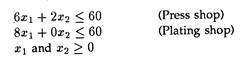
If there are only two variables, the problem can be solved by a simple graphical method. Where more than two variables are involved, we apply the ‘Simplex Method’.
Graphic Solution (Maximization):
Let us solve the same problem graphically. Here only two decision variables, i.e., x1 and x2 are involved. These variables are plotted along x-axis (horizontal) and y-axis (vertical).
ADVERTISEMENTS:
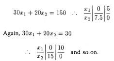
To plot the constraints on a graph, these are expressed in the form of the following equations:
8x1 = 60 (3)
![]()
Now OABCD in Fig. 5.1 is the convex region and the points in O,A,B,C,D are called the feasible solutions to the L.P. problem. There is a fundamental theorem of L.P. which states the objective function is optimized at one of the corner points, i.e., O,A,B,C,D. Thus for maximum profit only these corner points, also called basic feasible solutions, are to be evaluated.


The points can also be directly obtained from the graph.

Here Z = Rs. 450 (maximum at B when x1 = 5 and x2 = 15).
An alternative method for obtaining the optimal basic feasible solution is shown in fig. (5.2), which is same as fig. (5.1) with several dotted iso-profit lines, i.e., L1L1, L2L2, L3L3, etc. An iso-profit line is a graphical representation of all possible combinations of two products which give the same profit. These are parallel lines having the same slope. There may be infinite number of such lines. The farther an iso-profit line from the origin, the greater is the profit.
Here we select a reasonable profit and draw the objective function line relating to this profit. Next we pull the iso-profit line out of the solution space gradually till it touches the solution space at one extreme point only. Now we can find the optimum profit and the values of the decision variable from graph.
Z = 30x1 + 20x2 (objective function) is a linear equation of first degree. If we take different values of Z, e.g., 150, 300, 600 etc. and plot them on the graph, the lines will be parallel.
L1L1, L2L2, L3L3, are the iso-profit lines. L3L3 is touching the solution space 0ABCD at any one point, i.e., B(5,15).
... Z = Rs. 450 (optimum profit) and x1 = 5 and x2 = 15 (optimum product mix).
Graphic Solution: Minimization:
Let us discuss a minimization problem.
Problem 2
A person requires 10, 12 and 12 units of chemicals A, B and C respectively for his garden. A liquid product contains 5, 2 and 1 of A, B and C respectively per jar. A dry product contains 1, 2 and 4 units of A, B and C per carton. If the liquid product sells for Rs. 3 per jar and the dry product sells for Rs. 2 per carton, how many of each should be purchased in order to minimize the cost and meet the requirements?
Solution:
Let x1 = units of liquid product purchased and x2 = units of dry product purchased.
The objective function becomes:
Minimize Z = 3x1 + 2x2 (1)
subject to the following constraints

To plot the constraints on a graph, these are expressed in the form of the following equations:

Here the solution area lies beyond the lines (2)’, (3)’ and (4)’ as shown by the shaded area in Fig. (5.3).

Next we move the iso-profit line towards the origin till the last point on the boundary of the solution area is reached, i.e., B (here).
The co-ordinates of B can also be obtained by solving equations (2)’ and (3)’, as follows:
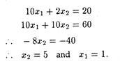
Now Z is minimum at B = 3 X 1 + 2 X 5 = Rs. 13. The coordinates of B can also be obtained from the graph directly.
The Simplex Method:
Complex L.P. problems cannot be solved by graphic solutions. For such problems we use the simplex method. Let us discuss a simple maximization problem.
Problem 1
The ABC Manufacturing Company can make two products P1 and P2. Each of the product requires time on’ a cutting machine and a finishing machine.

The number of cutting hours available per week is 390 the number of finishing hours available per week is 810. How much of each product should be produced in order to achieve maximum profit for the company?
Solution:
Let
x1 = Output of product P1;
x2 = Output of product P2;
x3 = Slack variable, i.e., unused cutting hours;
x4 = Slack variable, i.e., unused finishing hours;
and
Z = Optimum profit.
Now the objective function becomes: Maximize Z = 6x1 + 4x2 + 0x3 + 0x4 subject to the constraints:

As all the values of (Cj — Zj), i.e., index row of Pass II are either zero, or, negative, the optimum solution has been obtained.
The manufacturers must product 120 units per weeks and 150 units per week of P1 and P2, respectively to get the maximum contribution, i.e., Rs. 1320.
Calculations:
The process of calculation follows a few steps. These are explained below.
Starting Table:
Put the r.h.s. of equations (2) and (3) in CC’ and DC’ squares, respectively. Put the coefficients of x1, x2, x3 and x4 in equation (2) in CD’, CE’, CF’ and CG’ squares respectively. Similarly, put the coefficient of x1, x2, x3 and x4 in equation (3) in DD’,DE’, DF’ and DG’ squares respectively. Put the slack variables, x3 and x4, and their contributions 0 and 0, as show in in equation (1) in CB’, DB’, CA’ and DA’ squares, respectively.
Zj row calculations
EC’ square = 390 x 0 + 810 x = 0
ED’ square = 2 x 0 + 3 x 0 = 0 and so on.
Cj – Zj row calculations
FD’ square = 6 – 0 = 6 (i.e., AD’ – FD’)
FE’ square = 4 – 0 = 4 and so on.

Pass I Calculations:

Pass II Calculations:
Similar to Pass I
The index row (i.e., Cj – Zj) values in Pass II for the slack variables, i.e., X3 and X4, have a significant economic interpretation. Their absolute values, i.e., 2 and 2/3 here, show the amount of change in the optimal value of the objective function which would occur from relaxing the corresponding constraint by one unit.
This value is known as the ‘shadow price’. Hence we can say that if one more hour of cutting time were available, ABC manufacturing company could increase the profit by Rs. 2, i.e., the shadow price for cutting time is Rs. 2. Similarly, the shadow price for finishing time is Rs. 2/3.
Additional Aspects of the Simplex Method:
Big-M Method:
So far we have discussed about less than or equal to type constraints. But many problems have constraints of equalities, or, greater than or equal to inequalities. Let us take a problem and solve it.
Problem 1:
Maximize the profit function and give your comment:

Solution:
Introducing slack variables x4 and x5 and artificial variable x6, we have the objective function:

When the constraint if of the ≥ type, we must subtract a slack variable to get an equality constraint. To generate an initial basic feasible solution with such ≥ constraints, an “artificial variable” is added to each such constraints. Unlike slack variables, artificial variables have no economic meaning and are only used to establish an initial basic feasible solution.
As this variable has no economic meaning, we do not want it to appear in the final solution mix. Accordingly we assign a very large negative value in the objective function. In our Equation (1), M is an arbitrary large positive number.
Now see table 5.2. As, all the values of the final index (Cj – Zj) row are either negative, or zero, optimum solution has been reached.

... x1= 900, x2 = 1000, x3 = 0 and Z (maximum = 62,400.
Calculations are similar to the previous problem.
Problem 2.
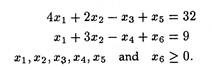
Use Big-M method to maximize Z = 6x1 + 4x2 subject to constraints
Give two different solutions, if the solution is not unique.
Solution:
Introducing slack variables x3 and x4, surplus variables x5 and artificial variable x6, we get the constraints as
And the objective function is: Maximize Z = 6x1 + 4x2 + 0x3 + 0x4 + 0x5 – Mx6
Now get the solution by eliminating big-M.
Minimisation Problem:
So long we have discussed about maximization problems. But in many practical situations, the objective function has to be minimized. Here we convert the minimization problem into a maximization problem by using the following expression.
Minimize Z = – Maximize (-Z).
Next we maximize (-Z) as before and take the negative value of maximize (-Z).
Problem 3.
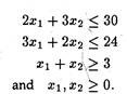
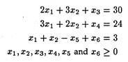
Use Big-M method to minimize Z = 15x1 + 12x2 subject to the constraints:
![]()
Solution:
Introducing surplus variables x3 and x4 and artificial variables x5 and x6, we get
Minimize Z = 15x1 + 12x2 + 0x3 + 0x4 + Mx5 + Mx6
subject to constraints
Now, Minimize Z = – Maximize (-Z). Here, Maximize (-Z) = -15x1 – 12x2 – 0x3 – 0x4 – Mx5 – Mx6.
Next apply Big-M method to solve maximize (-Z). The optimum value of minimize Z = the negative value of maximize (-Z).
The General Mathematical Statement of L.P. Model:

The Dual:
Every linear programming problem has a second complementary L.P. problem which is known as the ‘dual’. The original problem is called ‘primal’. The solution of the ‘primal’ can be obtained by solving either ‘dual’, or ‘primal’. If the ‘primal’ is a maximization problem, ‘dual’ is a minimization problem and vice versa.
Relationship between the Primal and the Dual:

Problem 1.
Primal Problem:
Maximize z = 60x1 + 80x2,

In both the cases z (max.) = α (min), y1 and y2 are the ‘dual’ variables. We can solve the ‘dual’ problems by graphic or simplex method.
Sensitivity Analysis:
After getting the optimum solution of a L.P. problem, we may study the changes in the optimum solution with changes in the parameters of the problem.
The following changes can be made:
(1) Change coefficients of the objective function.
(2) Change co-efficient of the variables on the l.h.s. of the constraints.
(3) Change the numbers on the r.h.s. of the constraints.
(4) Add/subtract new variables and
(5) Add/subtract constraints, etc.
This study is significant as it shows how sensitive is the current optimum solution to the changes in parameters. Management may be willing to know the range of variation of the parameters which does not affect the optimum solution under study.
This study of a L.P. problem is called “Sensitivity Analysis”. Most of the analysis is done by computer codes. We should be able to interpret the output from such codes, e.g., LPGOGO Code, etc..