Application of Linear Programming (With Diagram)

The below mentioned article provides an overview on the application of linear programming to the theory of firm.

The neo-classical theory of the firm analyses the problem of decision-making with one or two variables at a time. It is concerned with one production process at a time. The production function in linear programming goes beyond these limited fields of economic theory.

It takes into consideration the various capacity limitations and the bottlenecks which arise in the process of production. It makes a choice among the various complex productive processes so as to minimize costs or maximize profits.

Assumptions:

The linear programming analysis of the firm is based upon the following assumptions.

(1) The decision-making body is faced with certain constraints or resource restrictions. They may be credit, raw material and space constraints on its activities. Types of constraints, in fact, depend upon the nature of problem. Mostly, they are fixed factors in the production process.

(2) It assumes a limited number of alternative production processes.

(3) It assumes linear relations among the different variables which implies constant proportionality between inputs and output within a process.

(4) Input-output prices and co-efficient are given and constant. They are known with certainty.

(5) The assumption of additively also underlies linear programming techniques which mean that the total resources used by all firms must equal the sum of re-sources used by each individual firm.

(6) Linear programming, techniques further assumes continuity and divisibility in products and factors.

(7) Institutional factors are also assumed to be constant.

(8) For programming a certain period is assumed. For convenience and more accurate results, the period is generally short, though longer periods are not ruled out.

Given these assumptions, linear programming is used in the theory of the firm for the solution of the following problems:

1. Maximization of Output:

Let us suppose that a firm plans to produce a commodity Z, using X and Y inputs. Its objective is to maximize output. It has two alternative production processes, С (capital-intensive) and L (labour- intensive). The constraint is a given cost outlay MP, as shown in Figure 1. All other assumptions (noted above) relating to linear programming technique are applicable.

In the figure, units of input Y per period are measured along the vertical axis and units of input X per period are shown on the horizontal axis. If process С requires 2 units of input Y to every unit of input X, it will produce 50 units of commodity Z If the inputs of X and Y are doubled to 4 units of Y and 2 units of X, output is also doubled to 100 units of Z.

These combinations of X and Y, represented by a and b, establish the output scale along the capital-intensive process ray ОС. On the other hand, the same units (50) of good Z can be produced by process L by combining 3 units of X with one unit of Y. And 100 units of Z can be produced by doubling the inputs A and Y to 6 units of X and 2 units of Y.

These output scales are established along the labour-intensive process ray OL, as represented by input combination’s с and d. If the points a and с at the 50 unit output level on the linear rays ОС and OL are joined, they form an isoquant (shown dotted) IacS₁ .At the 100-unit output level, the corresponding isoquant is l₁bdS.

The cost outlay constraint is represented by the iso-cost curve MP and it places a limit on the production capacity of the firm. The firm can produce with either of the two available techniques С and L within the area represented by the triangle Obd. It is not possible tor it to produce outside this ‘area of feasible solutions’.

The optimal solution which maximizes the firm’s output will occur at the point where the iso-cost curve touches the isoquant with the highest output. In the figure, the iso-cost curve MP touches the isoquant i₁bdS at point b on the process ray ОС. It shows that the firm will use the capital-intensive technique С by using 4 units of input Y and 2 units of X and produce 100 units of commodity Z.

2. Maximization of Revenue:

Take another firm whose objective function is to maximize its revenue subject to certain constraints of limited capacities. Suppose the firm produces two products, X and Y. It has four departments each with a fixed capacity. Let these departments relate to manufacturing, assembling, polishing and packing the product which be designated as А, В, С and D. The problem is illustrated graphically in Figure 2.

The production of X and Y is subject to constraints A, B, C and D. Constraint A limits the production of X to OA. Constraint В limits the production of Y to OB. Constraint С limits the production of both X and У to ОС₁ and ОС respectively, while constraint D limits their production to OD₁ and OD. The area OATSRB shows all combinations of X and Y that can be produced without violating any constraints.

This is the area of feasible production within which X and Y can be produced, but there is no possibility of producing any combination at any point outside this area. The optimal solution can be found out by taking an iso-profit line within the feasibility zone.

An iso-profit line represents all combinations of X and Y which yield the same profit to the firm. The optimal solution lies on the highest iso-profit line EF in the polygon OATSRB at point S. Any point other than S lies outside the zone of feasible production.

3. Minimization of Cost:

The problem of minimization of cost was the first economic problem to be solved in linear programming. It relates to the diet problem. Suppose a consumer buys bread (x₁) and butter (x₂) at given market prices. Given the nutrient contents of each, how will the consumer minimise the cost of attaining the aggregate nutrients from various quantities of bread and butter. The problem is illustrated in Figure 3.

Bread (x₁) is measured along the horizontal axis and butter (x₂) is measured on the vertical axis. The line AB represents the combination of more butter and less bread, and CD represents the combination of less butter and more bread. The feasible solutions lie on or above the thick line AZD. The optimal solution is at point Z where the iso-cost dotted line RK passes through the point of intersection of AB and CD. The feasible solution may be at point A if bread were dearer or at D if butter were dearer but the optimal solution will occur at point Z in this problem.

Mathematical Note Graphic Solutions:

We attempt below a complete description and working of some problems of linear programming mathematically and graphically.

1. Maximisation of Revenue:

Take a firm that produces two products X and Y at given prices of Rs.12 and Rs.15 respectively for each unit. To produce product X, the firm requires 12 units of input A, 6 units of input В and 14 units of input C. Product Y requires 4 units of input A, 12 units of В and 12 units of input C.

Total available inputs in each case are 48 units of A, 72 units of В and 84 units of C. The input-output data for this problem is presented in Table 1.

Every linear programming problem has three parts to start with. They are as follows in terms of our problem stated above.

The Objective Function:

The objective function states that if the two products X and Y bring the revenue of Rs. 12 and Rs.15 per unit, how much of these products be produced so that the firm earns the maximum revenue.

It can be written as:

Мах: R = 12Х + 15Y

The Constraints:

The above table can now be transformed in the form of equations signifying the constraints or restraints within which the firm operates. These are known as structural constraints.

First, we take input A. The maximum available quantity of input A is 48 units. But the product of X and Y amounts of the two products cannot be greater than 48 units. Mathematically, since 12X + 4Y cannot be greater than 48 units, the constraints imposed by input A would be 12X + 4Y ≤ 48. With the same reasoning we can have the constraints in terms of inequalities for inputs В and C.

Thus the three structural constraints in our problem can be written as:

12 X + 4 Y ≤ 4Y … (1)

6X+ 12 Y ≤ 72…. (2)

14X+12 Y ≤ 84 … (3)

Where X and Y are our choice variables viz. units of inputs.

The Non-Negativity Constraints:

Then there are the non-negativity constraints in the linear programming problem which assume that there can be no negative values of variables in the solution of the problem. This means that the output of X and Y products can be zero or positive, but it cannot be negative. Thus the non­negative constraints of our problem are X ≥ 0 and Y ≥ 0.

The Graphic Solution:

For the Graphic solution we restate our problem:

Maximise R = 12X + 15Y

Subject to (i) 12X + 4Y £ 48

6X + 12Y £ 72

14X + 12Y £ 84

(ii) X³ ≥ 0 and Y³ ≥ 0

To represent each inequality graphically, we ignore the inequality sign (≤) in our equations and replace it by the equality (=) sign. We write equation (1) as 12 X + 4 Y = 48.

By assuming that the product X is produced only by utilizing the entire amount of 48 units of input A, we obtain

12X + 4Y = 48 (at the maximum)

or X = 4 (when Y = 0)

Similarly, assuming that the product Y is produced by utilizing the entire amount of 48 units of input A, we have

0 + 4Y = 48 or Y = 12 (when X = 0).

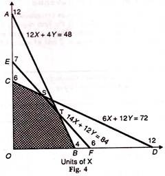
The equation 12X+ 4Y+ 48 is represented in Figure 4 by the line AB where OA =12 Y and OB = 4X. Any point on AB such as T satisfies the equation 12X + 4Y=48, while the area below and to the left of the line AB satisfies the inequality 12X+4Y≤48.

By solving the equation 6X + 12Y = 72 in a similar way, we obtain X =12, and Y=6. This is plotted in Figure 45.4 as the line CD which satisfies this equation where ОС =6Y and OD=12Y

And by solving the equation 14X+12Y= 84, we obtain X=6, and Y=7. Line EF in Figure 4 satisfies this equation where OE= 7Y and OF =6X.

The Feasible Region:

Figure 4 show that all the points in the shaded area bounded by the three lines intersecting each other would satisfy the three inequalities. At point S, line EF intersects line CD, and at T, line CD intersects AB. Thus the shaded area OBTSC which lies below and to the left of the three lines intersecting at points S and T satisfies the inequalities of the three equations.

This shaded area is called the feasible region of production and every point within the region or on the boundary of the region represents the feasible solution to our problem.

The Optimum Solution:

Out of the various points B, T, S, C which represents the feasible solution, we have to find out the optimal point that would maximise the revenue of the firm.

How to get this point algebraically? We know the coordinates of points В and С from Equations (1) and (2), whereby OB = 4X, and ОС = 67. In order to determine the coordinates of point T, we treat Equations (1) and (3) as simultaneous equations because the lines AB and EF representing them intersect at T and solve them as

12X+4Y= 48 … (1)

14X+12Y=84 … (3)

By multiplying Equation (1) by 3 and subtracting the latter from it, we have

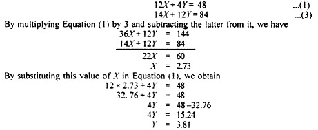
Thus the coordinates of point T are X= 2.73, and У = 3.81. Similarly, we can solve the coordinates of point S with Equations (3) and (2) which arrive at Z = 1.5 and Y = 5.25.

In order to find the optimal combination of X and Y, we substitute the values of X (Rs. 12) and У (Rs 15) into the values of the coordinates of the various comer points arrived at in the above paras.

At B, we have X = 4 and Y = 0, and substituting these in the objective function (Rs) R = 12X + 15 Y, we have

(Rs 12) (4) + (Rs 15) (0) = Rs 48…. (4)

At T, we have X = 2.73 and У = 3.81 and similarly obtain

(Rs 12) (2.73) + (Rs. 15) (3.81) = Rs. 89.91…. (5)

At S, we have X= 1.5 and Y = 5.25, and we obtain

(Rs 12) (1.5) + (Rs 15) (5.25) = Rs 96.75…. (6)

At C, we have Y = 6, and X = 0 and we get

(Rs. 12) (0)+ (Rs 15) (6)Rs 90 ….(7)

From the above Equations (4), (5), (6), and (7), we find that Equation (6) gives the maximum revenue of Rs 96.75. This shows that given the prices of the two products X and У, and given the amounts of inputs, the total revenue of the firm is maximized at point S. which is the optimal point subject to the given constraints.

Proving the Optimal Solution:

For the optimal solution to be correct, the total output produced must equal the total inputs available to the firm. We see above that the optimal point is S in Figure 45.4 where the firm maximizes its total revenue by producing 1.5 units of X and 5.25 units of У. In order to determine the total amount of each input used by the firm to produce the above units of X and У, we refer to columns (2) and (3) of Table 45.1.

To produce one unit of X, the firm uses the inputs 12A + 6В + 14С. And to produce one unit of У, it uses the inputs 4A + 125 + 12C. Since the firm produces 1.5 units of X and 5.25 units of Y, the various inputs used to produce these units are presented in tabular form below.

Adding the totals of the respective inputs, we find that the total amount of A input used is 18A + 21A= 39A, of input В is 9B + 63B= 72B, and of input С is 21C + 63С = 84С. The last column of Table 45.1 shows the maximum amount of input A available to the firm is 48 units, 72 units of input 5, and 84 units of input C. We find that inputs В and С are fully employed by the firm when it produces products X and Y at the optimal point S.

So far as input A is concerned, it is not fully employed because only 39 units are used by the firm and 9 units (48- 39) remain unutilized. That is why point T on the feasible boundary does not represent the optimal solution, it being the coordinate of Equations (1) and (3).

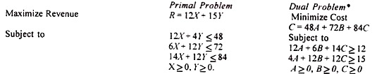
Dual of the Problem:

Every primal problem has its dual. In the above example, the primal relates to maximization of revenue. Its dual is minimization of cost.

To arrive at the dual of a primal problem, the following steps are required:

1. The columns and rows are interchanged.

2. The direction of inequalities in the constraints is reversed. If the primal has ≤ signs, the dual has ≥ signs.

3. The number of variables is reversed.

The primal problem given in Table 45.1 is set in the form of its dual as under:

2. The Diet Problem — Minimization of Cost:

The diet problem was the first economic problem to be solved by linear programming. Suppose a consumer buys bread and butter at given market prices. The problem is to minimize the cost of attaining the aggregate nutrients from the various quantities of the two foods.

Let x₁ and x₂ represent bread and butter respectively each containing the following contents of calories and grammes of protein. The nutrient contents of bread are 1000 calories and 50 grammes of protein per half kg; of butter, 2000 calories and 200 grammes of protein per half kg.

The standard diet should have 3000 calories and 200 grammes of protein per day. The market price of 500 gm. of bread is Rs 2 and of butter Rs 6 per 500 gm. This data is summarized in Table 2

The problem is to find the best diet according to the minimum nutritional standard as laid down in the last column of the above table and the least cost С indicated by (?). The total cost of diet is

The cost to be minimized is С which is a linear function of the two variables x₁ and x₂. The side relations 3 and 8 are inequalities which indicate the minimum nutritional standard of the given diet to be achieved. The problem is linear because the non­negative variables are to be minimized subject to linear inequalities.

The solution can be arrived at by any of the three conditions. For instance, the cost С can be minimized subject to one side relation: x₁ 2x₂ = 3. By solving it, we have x₁ = 3 and x₂ = 3/2 = 1.5. In Figure 5 this is shown by the line AB where OA = 1.5x₂ and OB = 3x₁.

The second side relation is 2x₁ + 8x₂ = 8, and by solving it we obtain x₁ = 4 and x₂=1. This is plotted in Figure 5 as the line CD which satisfies this equation where ОС = 1x₂ and OD = 4x₁. Thus in Figure 5, x₁ (bread) is measured along the horizontal axis and x₂ (butter) is measured along the vertical axis.

The line AB represents the combination x₁ + 2x₂ = 3 and CD represents the combination 2x₁+ 8x₂ = 8. The feasible solutions lie on or above the thick line AZD. The optimal solution is at point Z where the two lines AB and CD intersect.

In order to find out whether Z or any other point (A or D) within the feasible region AZD represents the feasible solution, we treat the two equations of the problem as simultaneous equations and solve them as:

X₁+ 2x₂ = 3……..(1)

2x₁+ 8x₂ = 8………….. (2)

By multiplying equation (1) by 4 and subtracting the latter from it, we have

4x₁ + 8x₂ = 12

2x₁ + 8x₂ = 8

2x₁ = 4

X₁= 2

Substituting the value of x₁ = 2 in (2), we get

2 x 2 + 8x₂ = 8

4 + 8x₂ = 4

8x₂ = 8-4

X₂ = 1/2

Thus the coordinates of point Z are x₁ = 2 and x₂ = 1/2. We know the coordinate of point A as x₂ = 1.5 and х₁ = 0, and of point D as x₁ = 4 and x₂ =0.

In order to find the optimal combinations of x₁ (butter) and x₂ (bread), we substitute the values of x₁ (Rs 2) and x₂ (Rs 6) into the values of the coordinates of the three points A, Z, and D.

At point A, we have x₂ = 1.5 and x₁ -0 and substituting these in the objective function C = 2x_t + 6x₂ we have

(Rs 2) (0) + (Rs 6) (1.5) = Rs 9…….. (3)

Similarly at Z, we have (Rs2)(2) + (Rs6)(1/2) = Rs 7 …….. (4)

At D, we have (Rs 2) (4) + (Rs 6) (0) = Rs 8…….. (5)

From the above equations, we find that equation (4) gives the minimum value of Rs 7. Thus the optimal solution of this diet problem is x₁ = 2, x₂ = 1/2, Z = 7 (minimum) which reveals that the daily minimum nutritional requirements of a person are met if he purchases 2 breads and 250 grammes of butter at a minimum cost of Rs 7 per day.

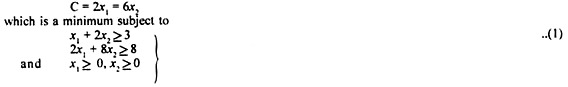
Its Dual:

Every minimization problem has its corresponding maximization problem, known as the dual. The primal of our diet problem is C = 2x₁ + 6x₂ which is a minimum subject to

This diet problem consists of providing 3000 calories and 200 gm of protein to be obtained from certain quantities of bread and butter at the minimum cost. Let y₁ and y₂ be the prices per unit of the two nutrients. The dual problem is to maximize P at the total value of the diet.

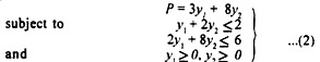
This shows that the expenditure on bread is y₁+ 2у which cannot be more than Rs 2 per half kg., and of butter it is 2у₁ + 8y₂ which cannot exceed Rs 6 per half kg.

In the dual, the primal is transposed in the side relations, i.e., in the primal problem the prices Rs 2 and Rs 6 are minimized and the minimum nutritional standard 3 and 8 are the side relations, whereas in the dual they appear in opposite places.

The solution to the dual given in equation (2) above is

Y₁ + 2у₂ = 2

2Y₁ + 8y₂ = 6

Multiplying equation (i) by 4 and subtracting equation (ii) from it, we get

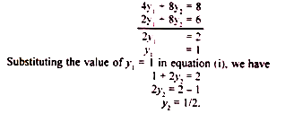
In order to find the optimal combination of y₁ and y₂, we substitute the values of y₁ (Rs 3) and y₂ (Rs 8) into the values of the coordinates of the corner points A and D in Figure. 6.

By solving the equation y₁ + 2y₂ = 2, the value of y₁ = 2 and of y₂ = 1 so that OA = 1y₂ and OB = 2y₁ in the Figure 6.

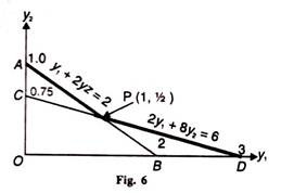
Similarly, the value of y₁ = 3 and of y = 3/4 or 0.75 from the equation 2y₁ + 8y₂ = 6 so that ОС = 0.75y₂ and OD = 3y₁ in the figure.

So at point A, we have y₂ = 1 and y₁ = О and substituting these in the objective function

P = 3Y₁+ 8Y₂ we have

(Rs 3) (0) + (Rs 8) (1) = Rs 8 ……. (iii)

Similarly at point P, we have (Rs 3) (1) + (Rs 8) (1/2) = Rs 7 …… (iv)

At point D, we have (Rs 3) (3) + (Rs 8) (0) = Rs 9 …… (v)

Thus we find that equation (iv) gives the minimum value of Rs. 7.

For all practical purposes the primal and dual problems must have the same solution, i.e., minimum Z = maximum P.

The solution to the primal problem was

x₁ = 2, x₂ = 1/2, Z = 7 (the minimum cost of diet).

The solution of the dual (2) works out at

Y₁ = 1, y₂ = 1 /2, P = 1 (the maximum value of diet).

In both the primal problem and its dual the same expenditure of Rs 7 per day is required for the optimal solution whether it is through the minimization of the cost of diet or maximization of the value of diet.

3. Profit Maximization Problem:

Let us take another linear programming problem relating to the maximization of profits. Suppose there is a small manufacturer who produces two products X and Y on two different machines, A and B. Product X requires 3 hours on machine A and 2 hours on machine B, whereas product Y requires 3 hours on machine A and 4 hours on machine B.

Machine A can be operated for 18 hours a day while machine В can be operated for 16 hours a day. The producer earns a profit of Rs 30 on each unit of product X, and Rs 40 on each unit of product 7. How many units of each product should he manufacture per day so as to have the maximum profit? For a better understanding the problem is presented in Table 3.

For the graphic solution, this linear programming problem can be restated as:

Maximise P = 30X + 40 Y (Rs)

Subject to (i) 3X + 3Y ≤ 18

or X + Y ≤ 6 ….(1)

2X + 4Y ≤ 16

X + 2Y ≤ 8 …. (2)

(ii) X ≥ 0, and 7 ≥ 0.

By solving the equation X + Y = 6 we have X = 6 and Y = 6. This is shown as line AB in Figure 7 where OA = 6Yand OB = 6X.

Similarly, by solving the equation X+ 2y = 8, we have X = 8 and Y= 4. This is shown as line CD in Figure 7, where ОС = 4 Y and OD = 8X.

The shaded area OBPC satisfies all the conditions of equations (1) and (2) and is the feasibility region. Every point in this region satisfies the mathematical inequalities.

In order to find out which of the corner points О, В, P or С represents the feasible solution where the profit is maximized, we treat the two equations as simultaneous equations and solve them as under:

X + Y = 6…. (i)

X + 2Y = 8…. (ii)

By multiplying equation

(i) By 2 and subtracting equation

(ii) From it, we get

Substituting the value of X = 4 in equation (i), we have

4 + Y = 6

or Y = 2

Thus the coordinates of point P are X = 4, and Y = 2. As already calculated above, the coordinates of point В are X = 6 and 7=0, and the coordinates of point С are X = 0 and X = 4.

In order to get the maximum profit, we calculate the profit at the corners of the feasibility region, i.e., O, B, P and С with the help of the values of these coordinates.

Profit at point О is zero.

Profit at point В = (Rs 30) (6) + (Rs 40) (0) = Rs 180

Profit at point P = (Rs 30) (4) + (Rs 40) (2) = Rs 200

Profit at point С = (Rs 30) (0) + (Rs 40) (4) = Rs 160

Thus the manufacturer will earn Rs 200 as the maximum profit (at point P) by producing 4 units of X and 2 units of 7per day. The optimal solution is, therefore, X = 4, Y = 2 and P = Rs 200 (maximum).