The Neoclassical Theory of Investment (With Diagram)

Let us make in-depth study of the Neoclassical theory of investment in an economy.

Introduction:

After Keynes, a neoclassical theory of investment has been developed to explain investment behaviour with regard to fixed business investment.

This theory is called neoclassical theory of investment behaviour because it is based on the neoclassical theory of optimal capital accumulation which is determined by relative prices of factors of production.

It may be recalled that fixed business investment refers to the purchase of machines, construction of new factories, warehouses, office buildings etc. by businessmen. The neoclassical theory of investment throws new light on the causes of fluctuations in investment which are responsible for occurrence of business cycles in a free market economy.

The neoclassical theory explains that at a particular time how much capital stock a firm desires to achieve. Further, according to this theory, rate of investment is determined by the speed with which firms adjust their capital stocks towards the desired level.

Because it takes time to build and install new machines, construct new factories, warehouses etc., the firms cannot immediately achieve the desired level of capital stock. Therefore, the firms have to decide with what rate or speed per period it makes adjustment in their stock of capital to attain the desired level of capital stock.

Firms use capital along with labour to produce goods and services for sale in the market. In deciding about the amounts of labour and capital to be used for production the firms are-guided by not only the prices of these factors but also the contributions they make to the production and revenue of the firms.

According to this neoclassical theory, investment, that is, addition to the stock of capital in an economy is determined by marginal product of capital (MPK) and user cost of capital which is also called real rental cost of capital. Marginal product of capital (MPK) measures the addition to the production by using an additional unit of capital, labour and technology remaining constant.

Due to the operation of the law of diminishing returns, marginal product of capital declines as more units of capital are used for production, the other factors being held constant. The user cost of capital will be explained in detail later, but it essentially stands for the rental for capital a firm owns or gets it on rent basis and measures the opportunity cost of the funds spent on production or purchase of a capital equipment.

The firms try to maximise profits or maximise the present value. Therefore, as long as the value of marginal product of capital (which are in fact marginal receipts or benefits it gets from the use of capital in production) exceeds the rental or user cost capital, it will be profitable for the firm to add to its stock of capital.

It will be maximising its profits when it has achieved the stock of capital at which marginal product of capital (MPK) equals user cost of capital. We can derive the desired stock of capital by using the neoclassical production function which is popularly known as Cobb-Douglas production function.

The Cobb-Douglas production function can be written as under:

Y = A K^α L^1-α

where Y stands for output, K for capital, L for labour and A is a parameter that measures the level of technology and α is a parameter that measures capital’s share of output. Marginal product of capital can be obtained by differentiating the production function with respect to labour. Thus,

Let r is the price or user cost of capital and p is the price of output. To maximise profits, a firm will equate the marginal product of capital to the real rental price (i.e. user cost) of capital (r/P).

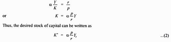
The equation (2) shows that the desired stock of capital (K*) depends on the size of output (Y₁), real cost of capital (r/p) . The equation (2) reveals that the higher the rental cost of capital (r), the lower will be the desired capital stock by the firm and vice versa. The equation (2) further reveals that the greater the expected output (Y_t) the greater the desired capital stock.

It may be noted that while in accelerator theory the changes in the stock of capital depends on the changes in output in neoclassical theory, the desired stock of capital depends not only on the planned output (Y_t) but also on the ratio of rental price of capital to price of output (r/p).

The rental or user cost of capital is determined by the price of capital goods, rate of interest, rate of depreciation and expected rate of inflation and the various features of tax system such as corporate tax rate, investment tax break etc.

The determination of the desired stock of capital is illustrated in Fig. 11.5 where on the X-axis we measure capital stock and on the Y-axis we measure MPK and rental cost of capital. As long as the marginal product of capital (MPK) is greater than the rental price or user cost of capital, it pays the firm to add to its stock of capital.

It will be seen from Fig. 11.5 that marginal product of capital is diminishing as there is increase in the stock of capital. Thus the firm will continue adding to the stock of capital (i.e. continue making investment) until the marginal product of capital (MPK) is equal to the rental price of capital.

If the rental price of capital is r₀, the firm continues investing until the capital stock K^r₀ is reached. K*₀ is the desired capital stock, given the rental price of capital equal to r₀ and for the given level of output (i.e. GDP) equal to, say, Y₁). It will be further seen from Fig. 11.5 that at the lower rental price of capital r₁, the firm’s desired capital stock will increase to K*₁.

Expected Output and Desired Capital Stock:

The equation (2) shows that desired capital stock depends on the level of output (Y_t). But this output level which determines the desired stock of capital is not the current output level but the expected output level for some future period in which capital stock will be used for production.

For some investment projects, future time for which output is planned may be few weeks or months away but for investment projects concerning power and steel future output level is planned many years ahead. However, current output level affects the expectations of future output level.

As the equation (2) above reveals that desired capital stock depends on the level of output, and in case of the economy as a whole, on the level of national income (GDP). When the level of output or national income is expected to increase the whole curve of marginal product of capital (MPK) will shift to the right as shown in Fig. 11.6. With this increase in the level of national product from Y₀ to Y₁, at the given rental cost of capital r₀, the desired capital stock increases from K₀ to K₁.

Rental Cost of Capital:

Since the desired capital stock and change in it depends on the rental cost of capital, it is important to know how rental cost of capital is estimated. If a firm finances its investment (that is, purchase of new capital goods) by borrowing, then rate of interest on the funds borrowed for investment purpose is an important element of rental cost of capital.

However, when inflation in the economy is occurring money value of capital rises over time, and as a result the firms make capital gain. Therefore, the real cost of using capital over a year is money interest payment minus the nominal capital gain. At a time when the firm has to decide to undertake investment, the nominal rate of interest is known to it but the rate of inflation is unknown.

At the best, the firm can have an expected inflation rate over the next years when it has to decide about investment. Therefore, the real cost of capital is estimated by nominal rate of interest adjusted for expected rate of inflation (π^e). Thus, expected real interest rate, that is, i – π^e is taken to be the real cost of borrowing funds for adding to the stock of capital.

Besides, capital undergoes wear and tear during its use for production in a year. Conventionally, depreciation is treated as a flat rate per year. Let this depreciation is d per cent per year. Thus, the rental cost or price of capital (r) is

r = i – π^e + d …(3)

Taxation and Rental Cost of Capital:

Besides real rate of interest and depreciation, taxes levied by the government also affect rental cost of capital. The corporation tax which is the tax on profits of the public limited companies and investment tax break or development rebate are the two important tax elements which influence the rental cost of capital.

Corporation tax is generally believed as a proportion, say, of the profits of the companies. The greater the corporation income tax the higher the rental cost of capital. The tax system of various countries also provides for investment tax credit to promote investment and development. Under investment tax credit scheme, the firms are allowed a certain rebate, say, 10 per cent of their investment expenditure, on the tax payable.

Thus investment tax break reduces the rental cost of capital.

If t_c represents the percent tax rebate on investment expenditure per year, then real cost of capital can be expressed as under:

r = i – π + d- t_c.

Capital Stock Adjustment:

The equation for desired capital stock, namely, K* α P/r Y_t shows that the desired capital stock depends on real rental cost of capital and the level of output (Y_t). When these variables change, the desired capital stock will change. Then the gap between the existing actual capital stock and the desired capital stock will emerge.

It always takes a good deal of time for the firms to make adjustment in the existing stock of capital to achieve the desired stock of capital. In other words, capital stock cannot be adjusted immediately and there are lags in the adjustment of actual capital stock to the level of desired capital stock.

Therefore, the firms make some adjustment in the capital stock in each period to finally attain the desired capital stock over time. If the firms attempt to adjust their actual capital stock immediately in addition to what may be called the direct cost of investment projects, the firms will have to bear adjustment costs.

The examples of adjustment costs are costs of temporary shutdown of plants to make the required additions, hiring of overtime labour, especially skilled labour, to complete the required construction work in a short period and costs incurred due to disruption of production. In view of these adjustment costs, it is optimal for the firms to make adjustment in the capital stock gradually over time to achieve the level of desired capital stock.

It may be noted that addition to the existing capital stock in each period is called investment.

Thus, investing (I_t) in a period can be written as:

I_t = K_t –  K_t-1

Flexible Accelerator Model:

There are a number of hypotheses about the speed at which firms attempt to make adjustment in capital stock over time. An important such hypothesis is called flexible accelerator model. According to this model, firms plan to invest, that is, add to the stock of capital per period to make only partial adjustment to fill up the gap between the desired capital stock and the existing capital stock.

However, according to this flexible accelerator model, the greater the gap between the current capital stock and the desired capital stock, the larger the firm’s rate of investment per period.

Thus, according to the flexible accelerator model, to make partial adjustment in each period the firms decide to undertake investment is each period, which is a fraction, say λ, of the total gap between the existing capital stock and the desired capital stock in each period. Let the capital stock at the end of the last period be denoted by K_t-1 , then the gap between the desired capital stock and the existing capital stock is K* – K_t-1.

Only fraction λ of the gap (K* – K_t-1) will be filled in each period to eventually attain the desired capital stock over time. Thus when the firm adds a fraction λ of the gap, K* – K_t-1 to the capital stock existing at the end of the last period (K_t-1), the capital stock at the end of the current period (K_t) will be

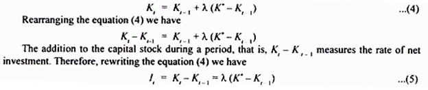
The equation (5) shows the partial and gradual adjustment of capital stock through investment in each period to reach the desired stock of capital over time. Only a part of the desired change in the capital stock is filled in each period by investment. Since in this flexible accelerator model investment in a given period is the result of changes in expected income or output during a number of previous periods, it shows a slower response of investment to changes in current period.

This implies that investment will be less volatile in the short run than is the case with the simple accelerator model which visualizes the response of investment to changes in current income wholly in one period. Empirical evidence corroborates the results of the flexible accelerator model as investment though volatile is not actually as volatile as simple accelerator model predicts.

The flexible accelerator model can also be modified to allow for changes in the speed with which investment is carried out (that is, the change in fraction λ is in fact the choice variable for the firm which is affected by such factors as the availability of credit, rate of interest, corporate tax rate, investment tax credit etc.

For example, if rate of interest is lower, more investment will be undertaken to fill the gap between the desired capital stock and the existing capital stock than would be the case if rate of interest is higher. Thus flexible accelerator model is quite consistent with the Keynesian theory that investment is negatively related to the rate of interest.

Graphic Illustration of Capital Stock Adjustment:

Capital stock adjustment through investment over time is illustrated in Figure 11.7 where along the horizontal axis we have shown the time and along the vertical axis we measure the capital stock. In the beginning of the period 1, the capital stock is K₁ and suppose the desired capital stock of the firm is K*. Thus K* – K₁ is the gap between the desired capital stock and the existing capital stock. Suppose the speed of capital stock adjustment is, λ = 0.5.

This implies that in each period one half of the desired capital stock and the existing capital stock is filled. Thus, in period t₁, the existing stock in the beginning of the period of K’ and given X = 0.5, the firm will add to the stock of capital, that is undertake investment equal to 0.5 (K* – K₁) = I₁ in period t₁.

Now in period t₂, the existing stock of capital will be K₂ and given λ = 0.5, the firm will undertake investment of 0.5(K* – K₂) = I₂ as shown by the shaded rectangle. It will be seen from Figure 11.7 that investment I₂ in period t₂ is less than investment I₁ in period t₁. This is because as net investment or addition to capital stock is made in period t₁ the gap between desired capital stock and the current capital stock is reduced and therefore the additional adjustment in capital stock in period t₂ becomes less in absolute terms.

Similarly, capital stock is adjusted through additional net investments in the next periods, in each period one-half (i.e., 0.5) of the remaining gap is filled until period t₇ when almost the whole gap between the desired capital stock and the existing capital stock is completely closed. It may be noted that the higher λ is, the faster the gap is filled.

In equation (5) we have derived an investment function that shows that investment depends on the desired capital stock K* and the existing capital stock K_t-1. Any factor that raises the desired capital stock will increase the rate of investment. Accordingly, increase in expected output and a reduction in rental cost of capital will cause increase in investment.

As seen above, rental cost of capital depends on nominal rate of interest, expected rate of inflation, corporate income tax, the investment tax credit which are important variables that determine the rental cost of capital will also affect investment in the economy.

To conclude our discussion of business fixed investment we have derived the neoclassical investment function of the following form:

I_n,t = F(Y^e, i_t, d, π^e, t_c, K_t-1) …(6)

This shows that net investment depends on expected level of output (Y^e), the various elements of rental or user cost of capital such as nominal interest rate i_t, expected rate of inflation (π^e), corporate income tax including investment tax credit, and the existing stock of capital. Given the existing stock of capital, an increase in expected output (Y^e), expected rate of inflation (π^e) and the investment tax credit will all increase investment. On the other hand, increase in nominal rate of interest (i_t) and the corporate income tax will cause net investment to decline.

The Neoclassical Theory of Investment: Role of Fiscal and Monetary Policies:

Now it is important to explain that the neoclassical theory of investment suggests what types of fiscal and monetary policies can promote investment. In our Keynesian analysis of fiscal policy we found that increase in government spending or cut in personal taxes will increase aggregate demand and national income and this will have favourable effect on marginal efficiency of capital which will tend to increase investment.

However, this high government spending and low personal tax policy also adversely affects investment because the increase in aggregate demand caused by it would raise the interest rate and crowd out private investment. This crowding out effect of high government expenditure and low personal tax policy tends to offset its favourable effect on investment via, increase in aggregate demand.

The neoclassical theory explained above suggests that if expansionary fiscal policy (that is, high government spending and low personal tax policy) is combined with a tax policy such as a greater investment tax credit will promote private investment. The investment tax credit is a sort of subsidy on investment and lowers the rental cost of capital.

As a result, the crowding out effect of expansionary fiscal policy via increase in nominal interest can be avoided. Besides, making adjustment in the rate of investment tax credit, it can be used as an alternative instrument to monetary policy as a means of stabilizing investment demand to achieve price stability as both investment tax credit and monetary policy work through change in the rental cost of capital.

In addition to above, the expansionary fiscal policy raises the level of income and expected output of the firms and will therefore raise the level of desired capital stock and hence stimulate investment. (Recall that K* = α p/r.Y_t

This beneficial effect of expansionary fiscal policy “may be quantitatively more important than any negative effect of a fiscal policy induced increase in interest rates. Which effect dominates depends on the importance of output growth versus the cost of capital as determinants of investment.”

However, as regards corporation tax, increase in it is likely to adversely affect rental cost of capital and will therefore discourage investment. On the other hand, reduction in corporation tax will increase profitability of investment through reduction in the rental or user cost of capital.

As regards monetary policy, it affects investment demand through its effect on real rate of interest. The neoclassical theory does not suggest any different monetary policy than that visualized in Keynesian and monetarist macroeconomic theories.

In neoclassical theory, expansionary monetary policy lowers interest rate which would reduce rental cost of capital and will increase the desired capital stock. Thus expansionary monetary policy stimulates private investment.