A Graphical Illustration of the Path to General Equilibrium

In this section we attempt to show how a simple economy with perfectly competi­tive production and factor markets will have an inescapable tendency toward a general equilibrium solution.

Assumptions:

1. Two substitute commodities are produced, X and Y, by two perfectly competi­tive industries (markets).

2. There are two factors, capital K and labour L, whose markets are perfectly competitive. The quantities of these factors are given (fixed supply).

3. The production functions are continuous, with diminishing marginal rate of factor substitution and decreasing returns to scale.

4. The industry producing X is less capital intensive than the industry producing y. The K/L ratio is smaller in industry X.

5. Consumers maximise utility and firms maximise profit.

6. The usual assumptions (of large numbers, homogeneous products and factors, and free entry and exit) of perfect competition hold.

7. The system is initially in equilibrium in all markets demand is equal to supply at a positive equilibrium price.

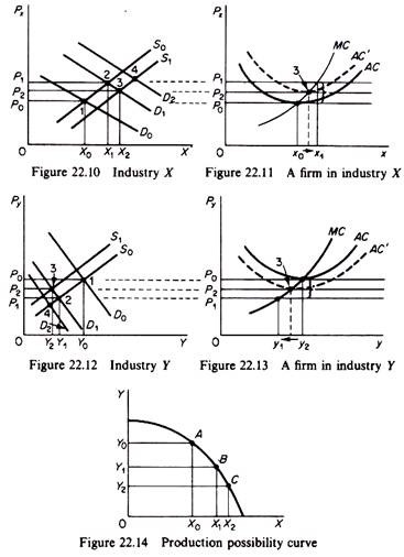
Assume that an exogenous change in consumers’ tastes shifts the demand for X outwards to the right, from D₀ to D₁ causing the price, in the short run, to rise from P₀ to Pix and the quantity sold to increase by X₀X_y units (figure 22.10).

Since X and Y are substitutes (ex hypothesis)’ one should expect the increase in the demand for X to be accompanied by a decrease in the demand for Y². The demand for y (figure 22.12) shifts to the left, its price drops and the quantity of Y sold decreases by Y₁ Y₀ units. (Note that with the assumption of given K and L, the economy cannot produce simultaneously increased quantities of both X and Y. Hence we must assume that an increase in the demand for X is accompanied by a decrease in the demand for Y there cannot be an increase in the demand for X without a corresponding concurrent decrease in the demand for Y, unless we allow for inflation.)

The increase in P_x creates excess profits for the producers of X (figure 22.11) and losses for the producers of Y (figure 22.13). Firms are thus induced to divert resources from the production of Y to the production of X. This is shown by the movement from point A to point B on the production possibility curve (figure 22.14). This shift reflects the effect of the change in consumers’ tastes on the decisions of firms.

The increase in P_x induces the producers of X to increase their quantity in order to maximize their profit, given the increase in marginal revenue. (The reaction of a typical firm in industry X is shown in figure 22.11.) Since every firm in the X industry faces the same price the output of each firm increases (each firm produces on the rising part of its AC). The sum of the increases in outputs of existing firms is equal to the increase X₀X₁ in figure 22.10.

In industry Y the opposite occurs. The fall in P_y induces firms to decrease their quantity. The reaction of a typical firm in industry Y is shown in figure 22.13. The sum of the decreases in output of the individual firms is equal to the decline Y₀ Y₁ in figure 22.12.

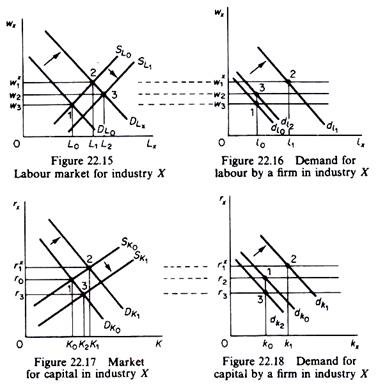
In the long run excess profits attract entry in industry X and induce exit of firms from industry Y. Entry and exit affect the demand for factors of production. The markets for labour and capital used in the production of X are shown in figures 22.15 and 22.17.

The expansion of production by existing firms and the entry of new firms in industry X increases the demand for labour and capital. The D_Lx and D_Kx curves shift outwards and w, and r_x rise. Employment of these factors rises in industry X (by L₀ L₁ and K₀K₁ respectively in figures 22.15 and 22.17). The demand for L and K by a single firm in industry X is shown in figures 22.16 and 22.18. The individual firm can buy any quantity of L and K at the prevailing market price. At the increased price w^x₁ the firm will demand l₁ of labour (figure 22.16), and at the increased price r^x₁ the firm will demand K₁, of capital (figure 22.18).

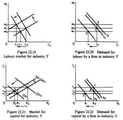
The situation in the labour and capital markets for the industry Y will be the reverse. The surviving firms in this industry will reduce their demand for both factors, while the exit of firms in the long run will further reduce the demand for these inputs. The situation for the factor markets in industry Y is shown in figures 22.19 and 22.21. The case of a single firm in industry Y is depicted in figures 22.20 and 22.22.

The above change in the demands for factors in the two industries leads to dis­equilibrium, because the prices of L and K have risen in the factor markets for industry X, while w and r have fallen in the factor markets of industry Y. However, in perfect factor markets the disequilibrium will be self-correcting, since in the long run there is perfect mobility of factors between the different markets. Thus the owners of L and K will withdraw their services from the Y industry and will seek to have them employed by firms in the X industry where w and r are higher.

The above reactions (mobility) of factor suppliers will result in an upward shift of the supply curve of factors in industry Y and a downward shift of the supply curves of factors in industry X. The shifts are shown in figures 22.15, 22.17, 22.19 and 22.21.

With the assumption that X is more capital intensive than commodity Y the prices of factors will not return to their original levels, w and r will be equalized in the two industries, but the wage level will be higher in the new equilibrium while the price of capital r will be lower in the final equilibrium (this is shown by the point 3 in figures 22.15, 22.17, 22.19, 22.21). The assumption of different factor intensities ((K/L)_x < (K/L)_y) has the following repercussions. The demand of the X industry for labour is stronger than the demand for capital.

The release of labour by industry Y is smaller than the rate required by X, while the release in capital is larger than the increased need for this factor by industry X. Thus overall the demand for labour will be higher than initially and w will rise. The opposite will occur in the market for capital, where the new equilibrium r will be lower than in the initial situation.

As a result of the new factor prices the individual firms in each industry will adjust their demands for labour and capital. In figures 22.16, 22.18, 22.20 and 22.22 the individual firms are in equilibrium at the points denoted by the digit (3).

The entry on firms in industry X shifts the supply curve downwards to Si (figure 22.10). The final equilibrium price of X is lower than in the short run, but higher than in the original equilibrium. The X industry is an increasing cost industry.

The exit of firms from industry Y shifts the supply of this industry upwards (figure 22.12). The final equilibrium price P₂ is higher than the short-run price P₁ but lower than the initial equilibrium level P₀. Industry Y is also an increasing cost industry.

Given the new product prices the individual firms will adjust (independently) their outputs. Firms in industry X will be producing an output lower than in the short run, but higher than in the initial equilibrium (figure 22.11).

Firms in industry Y will be producing an output higher than in the short run, but lower than in the initial situation (figure 22.13). The changes in w and r cause the LAC of firms in X to shift upwards (X is more labour intensive, and w has risen), and the LAC of firms in Y to shift downward (Y is more capital intensive, and r has fallen). Thus in the long run the firms earn just normal profits.

It should be noted that the above-described path towards a general equilibrium would be modified if, apart from the exogenous changes, we take into account pos­sible induced changes, generated by the adjustments in the system. For example, in our simple model we saw that in the new equilibrium wages were higher and the price of capital lower than initially.

If we accept the fact that wage earners have a higher propensity to consume than other factor owners, there will be a further (induced) increase in the demand for X, shifting the demand curve to D₂ in figure 22.10. From this point we can start tracing the additional changes in all other markets, as previously.

The above discussion is not a formal proof of the existence or stability of a general equilibrium. However, the assumption of perfect competition was adequate to enable us to see that the shifts in the supply and demand curves are not random, but precisely interrelated. The curves will continue to shift so long as disequilibria exist.

When an equilibrium is attained simultaneously in all markets and among all econo­mic decision-makers within the markets, we say that a general equilibrium exists throughout the entire economy, and the movement of curves will cease until another exogenous force disturbs the system.

In summary:

We started from an initial equilibrium, which was disturbed by an exogenous change in tastes. We traced the interactions of markets and individual decision-makers, in perfect product and factor markets. The system under our assumptions generated reactions which led to a new equilibrium. It should be stressed that this effect is certain only with perfectly competitive markets and contin­uous production functions with decreasing returns to scale.

If the system is not perfectly competitive we cannot be sure that a general equilibrium will be attained. The changes in initial conditions will be reflected in the various markets, but the economic signals are likely to be weaker. For example, in imperfect competition firms produce where P > MC. A shift in the demand for X will tend to increase production in this industry, but given P > MC, factors will tend to be under­employed in the X industry, and a rise in wages may create disequilibrium in the resource markets, leading to further disequilibria elsewhere in the system.