Price and Output Determination | Economics

The equilib­rium conditions of an individual firm under perfect competition are to be studied under two heads. They are: 1. Short-Run Equilibrium 2. Long-Run Equilibrium.

1. Short-Run Equilibrium:

A short period has two major characteristics:

(a) Fixed production scale:

In the short period a firm cannot change its scale of production. It has to increase its supply by utilising fully the existing machinery and capital equipment. So, it has to increase fixed and variable costs in such a period.

(b) No free entry or free exit of firms:

In the short period no new firms can enter into the industry, nor an old firm can go out of the industry. So, the number of firms in the industry remains the same.

Conditions of a short-run competitive equilibrium:

In such a short period there are two major conditions of equilibrium of a firm:

(a) P = SMC:

The total profits of a firm become maximum at the output where marginal cost is equal to marginal revenue. Under perfect competi­tion a firm is to sell all the units of its output at the same market price. For this reason market price becomes equal to a firm’s marginal revenue in this type of market.

So, it follows that the total profits of a competitive firm become maximum at the output level at which P=MC. So a competitive firm produces an output up to this level. It may be noted that in equilibrium position the marginal cost must be a rising one; otherwise there cannot be any stable equilibrium of a competitive firm.

(b) The Short-Run P and SAC—(Break-Even and Shut-Down Points):

In the short run, the competitive price may be greater than SAC, creating excess profits as no new firms can enter the industry. Sometimes it may be equal to AC and then the firm earns just normal profits, and this point (P=SMC=SAC) is called the break-even point as it equals TR with TC. Again, sometimes the competitive price may even be less than average cost yielding loss to the firm, provided it is greater than, or equal to, average variable cost.

If the market price is just equal to the average variable cost, the firm reaches what is called the shut­down point. Unless the position im­proves; or if the price goes below it, the firm will have to close down at this point. The short-run equilibrium output and price of a competitive firm is illus­trated in Fig. 4.

It shows that at price OP₁ (the de­mand curve being d₁d₁) the competitive firm produces OQ₁ units of output be­cause at this output level the price (OP₁ or Q₁d₁) is equal to the marginal cost (Q₁d₁). Here the price is greater than the average cost (Q₁d₁), creating an excess profit (Ld₁) is possible in the short run as no new firms can enter into the industry. If the price is lower, i.e., OP₂ (the demand curve being d₂d₂), the firm produces OQ₂ units of output, because at this output now the price (OP₂ or Q₂d₂) is equal to marginal cost (Q₂d₂).

Here the price is also equal to the average cost (Q₂d₂), giving the firm only normal profits. Such a point (P=SRMC=SRAC) is known as the break-even point (the point without either loss or profit, the normal profit being ignored). Again, if the price is still lower at OP₃ (the price line being d₃d₃), the firm would produce OQ₃ because at this output the present price (OP₃ or Q₃d₃) is equal to the marginal cost (Q₃d₃).

But, here the price is less than the average cost (Q₃T) creating a loss for the firm. Such a price is possible in the short run as it fully covers the average variable cost (Q₃d₃). The point (P=AVC) is called the shut-down point; the firm will shut down its business, unless the position improves or if the price falls below this short-run minimum limit of the average variable cost.

2. Long-Run Equilibrium:

A long period has also two characteristics:

(a) Variable Scale of Production:

In the long run a firm can change it scale of production. So, it has to increase only variable costs in the long run.

(b) Free Entry or Free Exit of Firms:

In the long run new firms may enter the industry or the existing firms can go out of it, depending on profits and losses.

Conditions of the long-run equilibrium of a competitive firm:

In such a long period there are also two important conditions of equilibrium of a competitive firm.

(a) P = LMC:

Even in the long run a competitive firm would produce an output up to that level at which price is equal to marginal cost which must be rising one. Although the equality of P and MC is an essential condition of the long-run equilibrium, it is not a sufficient one; another important condition is to be fulfilled for a stable long-run equilibrium.

(b) P = LAC (minimum):

The second condition is that the long-run com­petitive price must also be equal to average cost. It is obvious due to the fact that in the long run the total revenue of a competitive firm must cover its total cost. If the long-run price is greater than the average cost, the firm will make excess profits, which will attract new firms into the industry.

For this reason, the number of firms will increase, the total supply will be larger and the market price will fall to the level of average cost. So, the firm under consideration will incur a loss; as a result some firms will leave the industry, the number of firms will be smaller, the market supply will fall and the market price will rise again to the level of average cost.

Thus, it is clear that the long-run competitive price must equal both marginal cost and average cost, and the firm is then able to make only nor­mal profits. At this stage the average cost is the minimum (at the point of equality of P and LAC). So, in long-run equilibrium the competitive price be­comes equal to the minimum average cost.

Hence, the condition of the long- run equilibrium of a competitive firm becomes:

P=LMC=LAC (minimum).

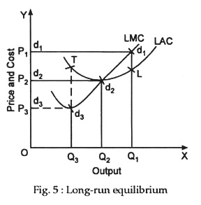
The long-run equilibrium of a competitive firm is shown in Fig. 5. Here at the output level OQ₁ the price OP₁ is equal to the marginal cost (Q₁d₁). This price cannot be stable as it is higher than the average cost (Q₁L). This price will attract new firms into the industry, causing an increase in market supply and a consequent fall in market price. If, on the other hand, market price is lower at OP₃, the firm produces OQ₃ units of output where the price is equal to the marginal cost (Q₃d₃).

This price also cannot be stable as it is lower than the average cost (Q₃T). But when the price is OP₂, the firm produces OQ₂. This price becomes stable as it is equal to both marginal and average costs (Q₂d₂). Here the average cost is the minimum. So, a competi­tive firm attains the long-run stable equilibrium position at the point of intersection of the three curves (d₂d₂, LMC and LAC), i.e., at the output level at which P=LMC=LAC (minimum).