Factor Price Equalisation Theory (With Obstacles) | International Economics

The factor price equalisation theory is an important corollary of the H-O theory of trade. If there is a free international movement of factors, the prices of the factors of production undisputably get equalised. However, the classical theorists as well as Heckscher and Ohlin had assumed an international immobility of factors. This led to the crucial question of how the international trade would affect the prices of the factors of production.

Heckscher, on the one hand, suggested that international trade in commodities would act as a substitute for the international mobility of factors leading to a complete equalisation of the costs or factor prices. Ohlin, on the other hand, recognised that the international trade might result in only an incomplete or partial equalisation of prices of factors. The writers like Samuleson (1948) and Lerner (1953) discussed the possibility of a complete equalisation of factor prices.

The factor price equalisation theory picks up the argument that the labour-abundant country specialises in the export of the labour-intensive commodity because labour is a relatively cheaper factor compared with capital. On the other hand, the capital-abundant country specialises in the export of capital-intensive commodity on account of capital being a relatively cheaper factor there. The pressure of international demand renders the abundant factor scarce and its price starts rising.

At the same time, the import of the commodities that require more input of scarce factor relieves the domestic pressure of demand for that factor, resulting in a fall in its price. The process of change in prices of factors will ultimately bring about an equality in the prices of factors. It is in this sense that free international trade in commodities acts as a substitute for the international mobility of factors.

1. Samuelson’s Analysis of Factor-Price Equalisation Theorem:

Samuelson’s analysis of the factor price equalisation is based upon the following assumptions:

(i) There are two countries, say A and B.

(ii) These countries produce two commodities, say X and Y.

(iii) The production of these commodities requires only two factors of production—labour and capital.

(iv) There is free competition both in the product and labour markets.

(v) There is an absence of tariff and transport costs.

(vi) The production function related to each commodity is identical and homogeneous of degree first. It implies the production is governed by constant returns of scale.

(vii) The factor-intensities are different for the two commodities. For instance, the commodity X is labour-intensive, while commodity Y is capital- intensive. It means there is an absence of reversal of factor intensity.

(viii) Capital and labour are qualitatively identical in the two countries.

(ix) The availability of factors is quantitatively different in the two countries. The country A is supposed to be labour-abundant whereas country B is capital-abundant.

(x) There is absence of complete specialisation. It means both the countries continue to produce both the commodities even after trade takes place between them.

(xi) The factor supplies are fixed in the two countries.

(xii) In each country, there is full employment of both the factors.

(xiii) There is no mobility of factors between the countries.

(xiv) The marginal-physical product of each factor is diminishing.

(xv) The tastes are identical in the two countries.

Before trade, there is low capital-labour ratio in country A and a high capital-labour ratio in country B. As trade commences, the labour-abundant country A exports the labour-intensive commodity X and country B exports the capital-intensive commodity Y. The export of labour-intensive commodity X by A creates relative scarcity of labour and consequent rise in wage rate. It also leads to a rise in capital- labour ratio.

On the opposite, the export of capital- intensive commodity by country B will result in its scarcity there. It will cause a rise in the price of capital (rate of interest) and a consequent fall in the capital-labour ratio. These relative changes in K-L ratio will continue until the K-L ratios in both the countries become exactly equal. Along with it, the prices of the two factors also undergo changes (rise in wage rate in country A and rise in interest rate of country B) in such a manner that there is ultimate equalisation of prices of two factors in both the countries.

2. Hicksian Analysis of Factor Price Equalisation Theorem:

J.R. Hicks attempted to provide a proof for the absolute factor price equalisation. He remained all the assumptions taken by Samuelson. It is assumed that price of labour is low in the labour- abundant country, while it is higher in country B which is capital-abundant. On the contrary, the price of capital is high in country A but it is low in country B.

After trade, country A exports labour- intensive commodity X and B exports capital-intensive commodity Y. l_x and l_y are the labour co-efficients for X and Y commodities and k_x and k_y are the capital co-efficient, w_a and w_b are the wage rates in the two countries, r_a and r_b are the rates of interest in these two countries. It is assumed that the unit cost of producing X and Y commodities becomes equal in the two countries after the determination of trade equilibrium.

Unit Cost of Commodity X:

l_x.w_a + k_x r_a = l_x.w_b + k_xr_b

Dividing both sides by k_x

(l_x/k_x) + r_a = (l_x/k_x) w_b + r_b

r_a – r_b = (l_x/k_x) w_b – (l_x/k_x) w_a

r_a – r_b = (l_x/k_x) [w_b – w_a] ….(i)

Unit Cost of Commodity Y:

l_y.w_a + k_y r_a = l_y.w_b + k_y r_b

Dividing both sides by k_y

(I_y/k_y) w_a + r_a = (l_y/k_y) w_b + r_b

r_a – r_b = w_b (l_y/k_y) – (l_y/k_y) w_a

r_a – r_b = (ly/ky)(w_b – w_a) …(ii)

From (i) and (ii)

r_a – r_b = (I_x/k_x) (w_b – w_a) = (l_y/k_y) (w_b – w_a)

If trade results in equalisation of factor-intensity in the two products X and Y and r_a = r_b, there will also be w_a = w_b. It shows that after-trade equilibrium results in the equalisation of factor prices.

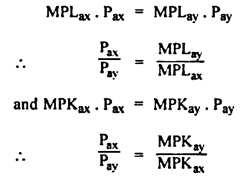
The relative factor price equalisation can be explained on the assumption that the value of marginal product (MP) of each factor within each country is equal before trade under the conditions of prefect competition in product and factor markets and constant return to scale.

Country A:

Country B:

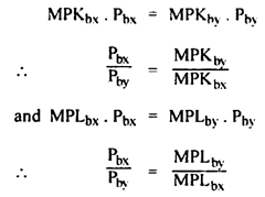
After trade takes place, there is equalisation of MPL and MPK in both the countries.

MPL_ax = MPL_bx, MPL_ay = MPL_by

MPK_ax= MPK_bx, MPK_ay = MPK_by

Hence (P_ax / P_ay) = (P_bx / P_by) respect of both the commodities in the two countries.

The relative equalisation of factor prices can be explained also through Fig. 8.3.

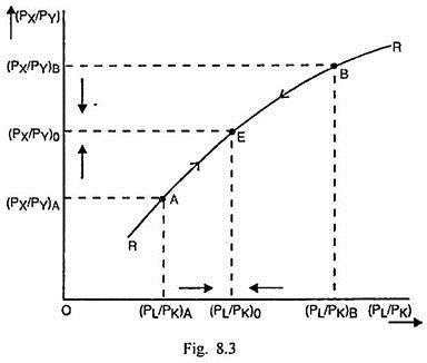
In Fig. 8.3, the factor-price ratio is measured along the horizontal scale and the commodity-price ratio is measured along the vertical scale. RR is the curve expressing the relation between the commodity price ratio and the factor-price ratio. Before trade, the labour-abundant country A is at the point A on the curve RR where the factor-price ratio P_L/P_K is low at (P_L/P_K)_A and the commodity price ratio is also low at (P_X/P_Y)_A because the labour-intensive commodity X is cheaper than the capital-intensive commodity Y.

On the other hand, the capital- abundant country B is originally at point B on the curve RR. At this point, both the commodity-price ratio and factor-price ratio are high at (P_X/P_Y)_B and (P_L/P_K)_B respectively. Country A has comparative advantage in commodity X and B has comparative advantage in commodity Y. Country A will export the labour-intensive commodity X and B will export the capital-intensive commodity Y.

The trade will lead to a rise in K-L ratio in country A and a fall in K-L ratio in country B. The increase in demand for labour relative to capital in A causes a rise in both the ratio of P_L to P_K and the ratio of P_X to P_Y. On the other hand, export of capital-intensive commodity Y by country B causes an increase in the demand for capital relative to labour. It brings about a fall in the ratio of P_L to P_K and also a fall in the ratio of P_X to P_Y.

These changes in factor-price ratio and commodity-price ratio continue until both the countries reach the point E on the curve RR. At this point, the factor- price ratio in both the countries becomes equal at (P_L/P_K)₀ and the commodity-price ratio gets equalized at (P_X/P_Y)₀. Thus trade results in the equalisation of relative factor prices in the two trading countries.

The relative factor price equalisation can be explained through the use of Edgeworth-type box diagram. First of all the effect of trade on factor- intensity and factor price ratio is analysed in the case of the labour-surplus country A.

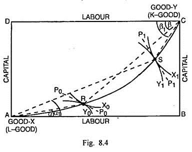
In Fig 8.4, the box ABCD is related to the labour-abundant country A. The longer horizontal scale and relatively short vertical scale signifies that country A is labour-abundant and capital-scarce. AC is the non-linear contract curve. Good X is labour-intensive good (L-good) and good Y is the capital-intensive good (K-good). A is the point of origin for the L-good X and C is the origin for K-good Y. X₀ and X₁ are isoquants related to good X and Y₀ and Y₁ are the isoquants related to good Y. Before trade, equilibrium takes place at R, which is the point of tangency between X₀. Y₀ and the factor-price line P₀P₀.

K-L Ratio in X = Slope of line AR = Tan α

K-L Ratio in Y = Slope of line RC = Tan β

As trade takes place, this country would specialise in the production and export of labour- intensive commodity X. The isoquant related to X commodity shifts to X₁. The equilibrium takes place at S where X₁, Y₁ and the factor price line P₁P₁ are tangent to one another.

K-L Ratio in X = Slope of line AS = Tan α₁

K-L Ratio in Y = Slope of line SC = Tan α₁

Since Tan α₁ > Tan α and Tan β₁ > Tan β it signifies that trade results in an increase K-L ratio in this labour-abundant country in respect of both the commodities. After trade, increased pressure of demand for labour results in an increase in price of labour relative to capital. This is shown by greater steepness of factor price line P₁P₁ than the original factor price line P₀P₀.

The changes in K-L ratio and factor price ratio in a capital-abundant country can be shown through Fig. 8.5.

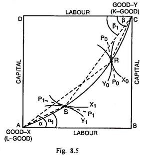
In Fig. 8.5 the box ABCD shows the capital-abundance of the country B. The vertical scale is longer than the horizontal scale. AC is the non­linear contract curve. Before trade, the original equilibrium occurs at R where the isoquant X₀ of good X and Y₀ of good Y are tangent to the factor price line P₀P₀.

The capital-intensity of two commodities at R is measured as:

K-L Ratio in X = Slope of line AR = Tan α

K-L Ratio in Y = Slope of line RC = Tan β

When trade takes place, this capital-abundant country specializes in the production and export of the K-good Y. As the production of Y is increased, the isoquant concerning this commodity shifts to Y₁. The equilibrium now takes place at S where the isoquants Y₁, X₁ and the factor price line P₁P₁ are tangent to one another.

The capital-intensity of two commodities at S is measured as:

K-L Ratio in X = Slope of line AS = Tan α₁

K-L Ratio in Y = Slope of line SC = Tan β₁

Since Tan α₁ < Tan α and Tan β₁ < Tan β, it signifies that trade results in a decrease in K-L ratio in respect of both the commodities. After trade, increased pressure of demand for capital causes an increase in the price of capital. This is reflected through the reduced steepness of the factor-price line P₁P₁ than the original factor price line P₀P₀.

The factor price equalisation after trade can be explained through Fig. 8.6.

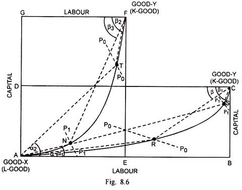
In Fig. 8.6 ABCD is the box related to the labour-abundant country A and AEFG is the box related to the capital-abundant country B. Before trade, the production takes place in country A at R and in country B at T. The capital-intensity of two commodities is measured below.

Before Trade:

K-L Ratio of X in country A=Slope of Line AR=Tan α

K-L Ratio of Y in country A=Slope of Line RC=Tan β

K-L Ratio of X in country B=Slope of Line AT=Tan α₂

K-L Ratio of Y in country B=Slope of Line TF=Tan β₂

When trade commences, the production in country A takes place at S. In country B, it takes place at N.

The capital-intensity of two commodities in two countries can be measured as:

After Trade:

K-L Ratio of X in country A=Slope of Line AS=Tan ∝₁

K-L Ratio of X in country A=Slope of Line SC=Tan β₁

K-L Ratio of X in country B=Slope of Line AN=Tan a₁

K-L Ratio of X in country B=Slope of Line NF=Tan β₃

Since Tan α₁ > Tan α and Tan β₁ > Tan β, the K-L ratio increases in both the commodities in country A. At the same time Tan α₁ < Tan α₂ and Tan β₃ < Tan β₂, there is a decrease in K-L ratio in both the commodities in country B.

After trade, K-L ratio in X commodity becomes exactly equal in both the countries because it is measured by the same Tan α₁. It happens because the points S and N lie upon the same line. In case of Y commodity too the capital-intensity is equal in both the countries because the line NF is parallel to the line SC. It means trade leads to equalization of capital-intensity of both X and Y in the two countries.

The increase in capital-intensity in country A occurs because of a rise in the price of labour relative to capital. On the opposite, the decrease in the capital-intensity in country B takes place because the price of capital rises relative to labour. Such changes in prices of the two factors bring about an equality in the factor price ratios in the two countries. In country A, originally the factor price ratio is represented by the slope of the factor price line P₀P₀ which is less steep.

After trade, it becomes steeper as shown by the factor price line P₁P₁. It signifies that there is an increase in price of labour relative to capital. In country B, the factor price line P₁P₁ after trade becomes less steep compared with the original factor price line P₀P₀. It is on account of the fact that capital becomes costly relative to labour. Since the slope of factor price line P_1­P­₁ at S is exactly equal to the slope of factor price line P₁P₁ at N (these factor price lines are parallel), the factor price ratios have been equalized through trade.

3. Lerner’s Analysis of Factor Price Equalisation Theorem:

Lerner has attempted an analysis about the factor price equalisation theorem on the basis of a series of assumptions.

(i) There are two countries A and B.

(ii) Each country can produce two goods X and Y, given the factor endowments and techniques of production.

(iii) There are two factors of production— labour and capital.

(iv) The production functions are linear homogenous in both the countries.

(v) Country A is labour-abundant and B is capital-abundant.

(vi) There are the conditions of perfect competition in both the countries.

(vii) There is absence of transport costs.

(viii) Commodity X is labour-intensive while commodity Y is capital-intensive.

(ix) There is no factor-intensity reversal.

In the labour-abundant country A, originally price of labour is lower relative to that of capital. On the opposite, the price of capital is lower in country B than that of labour. Consequently, country A will produce and export labour-intensive commodity X. As there will be greater substitution of labour for capital, the price of labour will rise and that of capital will decline resulting in equalisation of factor prices.

Similarly the capital- abundant country B will specialise in production and export of capital-intensive commodity Y. The substitution of capital in place of labour will increase the price of capital in this country. Ultimately, the factor prices ratio in this country will also get equalised.

However, if there is factor-intensity reversal i.e., X is labour-intensive in country A but capital- intensive in country B, both the countries will produce it through different techniques. But as they cannot export the same product to each other, the factor price equalisation will fail to take place.

4. Kindelberger’s Analysis of Factor Price Equalisation Theorem:

Kindelberger has explained the factor price equalisation by involving factor proportions, product prices and factor prices.

In this regard, he has relied upon the figure given below:

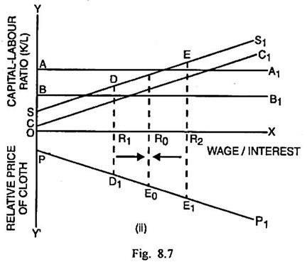
In Fig. 8.7 Part (i), wages and interest are measured along the horizontal scale and capital- labour ratio (K/L) is measured along the vertical scale. The horizontal line AA₁ and BB₁ measure factor proportions in the capital-abundant country A and labour-abundant country B respectively. SS₁ is the schedule related to capital-intensive good steel and CC₁ is the schedule related to labour- intensive good cloth. In Part (ii) of the Fig. 8.7, relative price of cloth is measured along the vertical scale.

The curve PP₁ measures relative price of cloth. The domestic demand conditions determine the production of steel and cloth before trade. Wage rate is lower in country B than in country A, whereas the rate of interest is higher in B than in A. The relative price of cloth in A is R₁D₁ and it is R₂E₁ in country B. As trade takes place, the wage rate will rise in country A and fall in country B. The interest rate, on the other hand, will fall in country A but rise in country B. The relative price of cloth in both the countries will tend to approximate to R₀E₀, when wage-interest ratio becomes equal at R₀.

5. Sodersten’s Analysis of Factor Price Equalisation Theorem:

Bo Sodersten recognises that the free trade can lead to the equalisation of relative factor prices in two countries. Neither country specialises completely. It can be explained through Fig. 8.8. In this figure, factor price ratio (w/r) is measured along the horizontal scale. In Part (i) of the Fig, the commodity price ratio (P_x/P_y) is measured along the vertical scale. In part (ii) of the Fig, the factor intensity (K/L) is measured along the vertical scale.

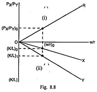
Given that there is absence of complete specialisation in both countries A and B, the line OR in Part (i) of Fig. 8.8 shows a common factor price ratio (w/r)₀ and the common commodity price ratio (P_x/P_y)₀. In Part (ii) of Fig. 8.8.., the lines X and Y represent the capital-intensity of X and Y commodities respectively. The commodity Y has greater capital-intensity (K/L)₁ than the commodity X, in case of which capital-intensity is low at (K/L)₀.

If there is complete specialisation in one or both the countries, there cannot be equalisation of absolute or relative factor prices. It can be shown through Fig. 8.9.

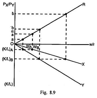
Under autarchy, the range of relative commodity prices for country A is indicated by aa. In case of country B, the range of relative commodity prices is denoted by bb. These two ranges do not overlap; therefore, at least one of the two countries must specialize completely. As both countries specialise completely, the free trade commodity price ratio is α which lies outside the autarchy price ranges.

The relative wage rate in country A cannot rise above w_A, whereas that of country B cannot fall below w_B. In such conditions, there cannot be relative factor price equalisation. So there cannot also be absolute factor price equalisation.

Obstacles to Factor Price Equalisation Theory:

The factor price equalisation theory developed by Samuelson has been found to be deficient by several economists including Meade and Ellsworth. They raised serious doubts about the validity of this theory on account of highly restrictive and unrealistic assumptions. They believe that there can only be partial equalisation of factor prices. There are serious obstacles to a complete equalisation of factor prices in the trading countries.

Such obstacles are discussed below:

(i) Tariff and Non-Tariff Barriers:

The theory rests upon the assumption that there are no tariff and non-tariff barriers to trade. In actual reality, such barriers do exist. It was on account of them that Ohlin ruled out the possibility of complete equalisation of factor prices.

(ii) Transport Costs:

The factor price equalisation theory takes another unrealistic assumption that transport costs are absent. In fact, the import and export of commodities do involve transport costs, which not only have restrictive effect on the product mobility but may also affect the comparative advantages of the trading countries. The existences of transport costs are likely to prevent the equalisation of factor prices.

(iii) Complete Specialisation:

This theory assumes that the trading countries are engaged in the production of both the commodities. In other words, there is only partial or incomplete specialisation. When the trading countries are of unequal size, there is possibility that there is complete specialisation in at least the smaller country. In the event of complete specialisation, there is little possibility of complete factor price equalisation.

(iv) Identical Production Function:

Samuelson’s factor price equalisation theory assumes that production functions are identical in the two trading countries. Even if the two countries have the same resources, yet their productive capacities are different because of natural, technical and sociological differences between them. The diversities in their production functions may create hindrance in the equalisation of factor prices.

(v) Absence of Perfect Competition:

This theory rests upon the assumption that there are the conditions of prefect competition in the product and factor markets. In actual reality, the prefect competition does not exist. In the real market situations like oligopoly or monopolistic competition, there are rigidities in the product and factor markets that prevent the possibility of equalisation of factor prices.

(vi) Increasing Returns to Scale:

The factor price equalisation theorem assumes that there is a first-degree homogeneous production function, which implies that the production is governed by the constant returns to scale. If the economies of scale are present, according to Meade, the theory will become invalid for two reasons. Firstly, it will result in the emergence of monopolies and consequent breakdown of the apparatus based on the assumption of perfect competition. Secondly, the increasing returns to scale will lead to complete specialisation, which again rules out the possibility of equalisation of factor prices.

(vii) Changes in Factor Supplies:

The theorem takes the assumption that the factor supplies remain fixed in the trading countries. In actual reality, however, there are changes in factor supplies and these changes will create difficulties in the equalisation of factor prices.

(viii) Dynamic Conditions:

The factor price equalisation theory assumes static conditions such as fixed factor endowments, techniques and same taste pattern in the trading countries. In the actual dynamic conditions, the continuous changes take place in all the relevant factors and variables and many often it is found that the differences in factor prices get widened rather than being eliminated.

Such a trend has been confirmed by economists like Kindelberger, Myrdal and Sodresten. In the words of Kindelberger, “…trade between developed and less developed countries widens the gap in living standards (the factor prices such as wages) rather than narrows, and it is evident after centuries of trade that there are still poor as well as rich countries.

(ix) Multi-Country, Multi-Commodity and Multi-Factor Trade:

The theorem can deal efficiently only in respect of trade involving two countries, two commodities and two factors. The theory is likely to become indeterminate in the multi-country, multi-commodity and multi-factor trade situation. If the number of productive factors exceeds the number of commodities, the theory breaks down completely.

(x) Factor-Intensity Reversal:

This theory assumes that there is an absence of factor intensity reversal. It means the labour-surplus country will export only labour-intensive commodity and the capital-surplus country will export the capital- intensive commodity. If there is reversal of factor intensity, the factor price equalisation theorem will fail to hold. If the labour-surplus country A specialises in the labour-intensive commodity X, the absolute and relative wage rates will rise in this country.

If country B specialises in commodity Y but produces it thorough labour-intensive method, the demand for labour will increase even in this country resulting in a rise in the absolute and relative wage rate. As the wage rates rise in the two countries, whether the difference in absolute and relative wage rates will rise, fall or remain unchanged, will depend on the rates at which wages increase in the two countries. Thus the factor- intensity reversal can result in the invalidation of the factor price equalisation theory.

The above arguments suggest that factor price equalisation cannot take place in actual dynamic realities. It, however, does not mean that the theorem is completely invalid. It only means that the assumptions of this theorem, being unrealistic, lead to an unrealistic conclusion.

There is little doubt that the movement of products from one country to another can at least reduce the factor price differentials. In the absence of trade, such differences are likely to be considerably large. In the words of Robert Heller, “…the effect of international trade may be considered as a ‘ leaning against the wind’ in that factor price differentials would be even larger in the absence of trade.”