The Equilibrium of a Multiproduct Firm

In this article we will discuss about the equilibrium of a multiproduct firm, explained with the help of suitable diagrams.

Introduction to Equilibrium of a Multiproduct Firm:

Let us consider the simplest case of a multiproduct firm in which a firm uses a single input X for the production of two goods, viz., Q₁ and Q₂.

The firm’s production function in implicit form can be written as:

H(q₁, q₂,x) = 0                           (8.162)

where q₁, q₂ and x are respectively the quantities of Q₁, Q₂ and X.

Let us assume that (8.162) can be solved explicitly for x:

x = h(q₁,q₂)                               (8.163)

(8.163) gives us the cost of production, in terms of input quantity x, as a function of the output quantities q₁ and q₂.

Now, the firm may use many different combinations of q, and q₂ by using a particular quantity of input X. The curve that connects these (q₁, q₂) combinations is called the product transformation curve (PTC). The equation of the PTC for x = x₀ = constant is

x₀ = h(q₁,q₂).                           (8.164)

We have presented three of a family of PTCs in Fig. 8.28 for three particular values of x, viz., x₁, x₂, and x₃.

Let us now state the assumptions upon which we shall base further discussions of the model.

These assumptions are:

(i) The firm is a profit-maximiser. That is why marginal products (MPs) of input X in the production of both Q) and Q₂ should be positive.

(ii) x in (8.163) is an increasing function of q) and q₂, which implies that the marginal costs (MCs) of producing both the goods are positive. Also, (8.163) is defined for x ≥ 0 and q₁ , q₂ ≥ 0. The assumption that x is an increasing function of q₁ and q₂ also implies, by the inverse function rule, that qi and q₂ are increasing functions of x, i.e., MP_X in the production of both Q₁ and Q₂ is positive.

(iii) The product transformation curves (PTCs) that would be obtained for different values of x, are negatively sloped and concave to the origin as have been shown in Fig. 8.28. This implies that (8.163) is regular strictly quasi-convex. The slope of a PTC has been assumed to be negative, for a particular quantity of input X may produce more (or less) of Q| only when it has to produce less (or more) of Q₂.

The numerical slope of a PTC at any point on it, is called the marginal rate of product transformation of Q₂ into Q₁ (MRPT_Q1,Q2) at that point.

The PTCs have been assumed to be concave to the origin because it has been observed empirically that as the firm goes on transforming Q₂ into Q₁, i.e., as it moves downward towards right along a PTC, the MRPT_Q1,Q2 or the numerical slope of the curve increases. In accordance with the definition of MRFT given above, we may write

Now, taking the total differential of (8.163), we have

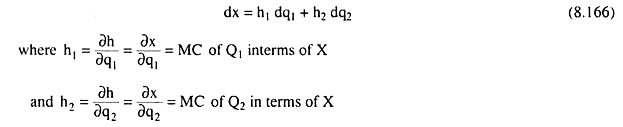
Since dx = 0 for movements along a PTC< we have

That is, the MRPT at a point on a PTC equal the ratio of the MCs of the two goods (Q₁ and Q₂) in terms of X.

Alternatively, MRPT can be expressed in terms of the marginal products (MPs) of input X.

The inverse-function rule gives us

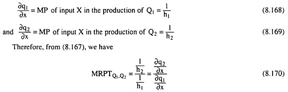
That is, the MRPT_Q1,Q2 equals the ratio of the MPs of input X in the production of Q₂ and Q₁.

Types of Equilibrium of a Multiproduct Firm:

(a) Constrained Revenue Maximisation:

If the entrepreneur sells his goods, Q₁ and Q₂, at fixed prices p, and p₂, his revenue (R) equation would be

R = p₁q₁ + p₂q₂                              (8.171)

If the entrepreneur specifies the amount of revenue that he wants to earn as, say, R = R₀, his revenue equation (8.171) would become

R₀ = p₁q₁ + p₂q₂                           (8.172)

which may be considered to be his iso-revenue equation. This equation would be represented by a straight line of slope = p₁/p₂ negative, and the horizontal and vertical intercepts of this line would be R₀/p₁ and R₀/p₂, respectively. We have shown three such iso-revenue lines for R = R₁, R₂ and R₃ in Fig. 8.28. They are parallel straight lines, given the prices of the goods.

If the firm wants to maximise revenue (R) subject to the input constraint

X₀ = h(q₁,q₂)                 [(8.164)]

then, to derive the conditions for such maximisation, we have to form the relevant Lagrange function:

Where λ is an undetermined Lagrange multiplier.

The first-order conditions (FOCs) for constrained revenue maximization are

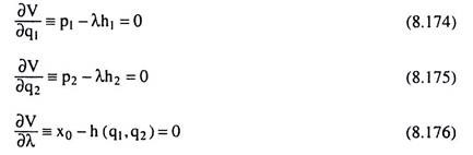
Transposing terms of equations (8.174) and (8.175) and dividing the former by the latter, we obtain

Or, substituting from (8.170), we have

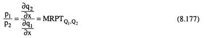
The FOC for constrained revenue maximisation as given by (8.177), therefore, tells us that MRPT must be equated with the fixed price ratio. Geometrically, since MRPT is the numerical slope of the product transformation curve (PTC) and is that of the iso-revenue lines, constrained revenue maximisation occurs at the point of tangency between the given PTC and an iso-revenue line.

Given the PTC or given the input constraint, the firm, at this point, would be on the highest possible iso-revenue line, i.e., on the highest possible level of revenue. In Fig. 8.28, if the input constraint is given to be x₃, the firm would maximise revenue subject to this constraint at the point of tangency F₃ between the PTC for x = x₃ and the iso-revenue line for R = R₃.

The FOC may also be written as

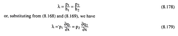
Since p₁/h₁ = p₁(∂q₁/∂x) is the increase in revenue per unit increase in x, or, the marginal revenue product of x (MRP_X), in the production of Q₁, and p₂/h₂ = p₂(∂q₂/∂x) is the increase in revenue per unit increase in x or, the MRP_X, in the production of Q₂, the FOC given by (8.178) requires the revenue maximising firm to distribute the use of the given amount of X between the production of the two goods in such a way that the MRP_X may become the same in the production of each good.

Again, since p₁(∂q₂/∂x) is the value of the marginal product of input X(VMP_X) in the production of Q₁ and p₂ (∂q₂/∂x) is the VMP_X in the production of Q₂, the form of the FOC as given by (8.179) requires that the revenue maximising firm should distribute the use of the given quantity of input X between the production of two goods in such a way that the VMP_X may become the same in the production of both the goods.

It may be noted here that, if pi and p₂ are given and constant, then MRP_X and VMP_X would be identical in the production of each good. Let us now come to the second-order condition (SOC) for constrained revenue maximisation. This condition states that the relevant bordered Hessian determinant be positive, i.e.,

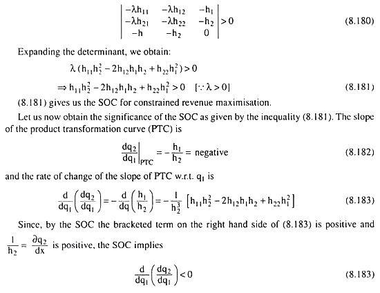
which implies that the derivative of the numerical slope of PTC, i.e., derivative of –(dq₂/dq₁) w.r.t. q₁ is positive, which, in its turn, implies that the PTC is concave to the origin at the point of tangency where the FOC has been satisfied. Since we have already assumed PTCs to be concave to the origin, the SOC may be considered to have been satisfied here.

We have so far assumed that the firm wants to maximise revenue subject to an input constraint. But it may be the other way round. That is, the firm may decide to minimise its use of input X subject to a revenue constraint.

In this case, the firm’s iso-revenue line would be specifically given and the firm would want to remain at that point on the line where it would reach the lowest product transformation curve (PTC), or, where the minimum amount of input X would be used.

Here also, the firm would achieve optimisation at the point of tangency between the given iso-revenue line and a PTC, and here also, the FOC and the SOC would be the same as those in the constrained revenue-maximisation case.

If the PTCs are strictly concave to the origin, every point of tangency between an iso-revenue line and a PTC represents a solution of both a constrained revenue-maximisation and a constrained input-minimisation problem. If we join all such points of tangency and the point of origin, O, by a curve (like OE in Fig. 8.28), then this curve would give us what is known as the firm’s output expansion path.

(b) Profit Maximisation:

In this model, the firm’s profit (π) function would be obtained as

π = p₁q₁ + p₂q₂ – rx (where r is the price of input X)

= p₁q₁ +p₂q₂ -rh(q₁, q₂)

= π(q₁,q₂)                                                  (8.184)

Here pi and p₂ are the given prices of Q₁ and Q₂ and r is the given price of input X. The FOCs for maximum profit would be obtained if we set the partial derivatives of π w.r.t. q₁ and q₂ equal to zero. Therefore, the FOCs are

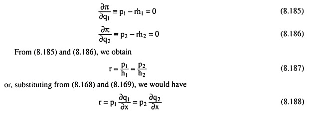
The FOCs for profit-maximisation as given by (8.187) and (8.188) require, like those of constrained revenue maximisation or cost minimisation [as given by (8.178) and (8.179)], that the MRP_X ≡ VMP_X should be equal in the production of both the goods, but profit-maximisation requires, in addition, that the MRP_X ≡ VMP_X for both the goods should be equal to r which is the price of input X.

Therefore, we may conclude that profit-maximisation ensures constrained revenue maximisation or input minimisation, but the latter does not ensure the former, because the latter does not lead to profit-maximising conditions p₁ = rh₁ and p₂ = rh₂, i.e., the equality between price and marginal cost for each good, as given by (8.185) and (8.186).

Let us now come to the second-order conditions (SOCs) for profit maximisation.

These conditions require that the principal minors of the determinant:

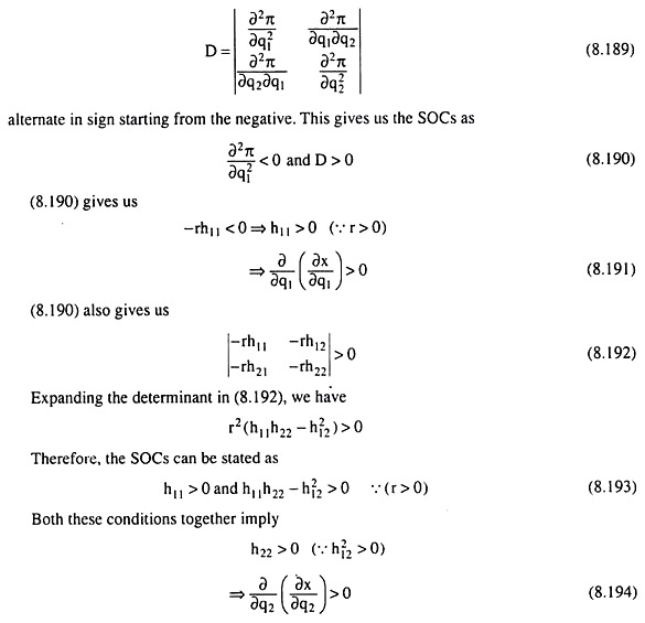
The SOCs (8.191) and (8.194) for profit maximisation give us that the MCs of both the goods, ∂x/∂q₁ and ∂x/∂q₂ and rise as q₁ and q₂ increase respectively. In other words, the MC curves of both the goods should be upward sloping towards right.

In terms of MPs, the second order condition states that as qi and q₂ rise, i.e., as x rises, the reciprocals of the MCs of the goods decrease, i.e., and decrease, i.e., ∂q₁/∂x and ∂q₂/∂x decrease, i.e., MP_X in the production of both the goods decreases, or, p₁ ∂q₁/∂x and p₂ ∂q₂/∂x decrease, i.e., the values of marginal product of X in the production of both the goods decrease.

SOCs (8.193) require that the production relation (8.163) be strictly convex in the neighbourhood about a point at which the FOCs (8.188) are satisfied. If (8.163) is strictly convex throughout, any maximum achieved will be a global maximum.