Investment Demand in Macroeconomics: An Overview

The below mentioned article provides an overview on the investment demand in macroeconomics. The study of investment will help in better understanding of fluctuations in the economy’s output.

Introduction:

We study investment to better understand fluctuations in the economy’s output. We have seen simple investment function relating investment to the real interest rate: I = I (r). That function states that, an increase in the real interest rate reduces investment. We now want to see more closely the theory behind this investment function.

There are three types of investment spending. Business fixed investment includes the plant and machine that business buy to use in production. Inventory investment includes those goods that businesses put aside in stores, including inputs, finished goods and work-in-progress. Residential investment includes the new housing that people buy to live in and that landlords buy to rent out. Here we build models of each type of investment to explain these fluctuations.

As we develop the models, it is useful to keep in mind the following questions:

Why is investment negatively related to the interest rate?

What causes the investment function to shift?

Why does investment rise during booms and fall during recessions?

At the end of our discussion, we return to these questions and summarize the answers that the model offer.

Business Fixed Investment:

The standard model is called the neo-classical model of investment. This model examines the benefits and costs to forms of owing capital goods. The model shows how the level of investments — the addition to capital stock — is related to the marginal product of capital (MP_K), the interest rate, and the tax rules affecting firms.

Let us imagine that, there are two kinds of firms in the economy. Production firms produce goods and services using capital that they rent. Rental firms make all the investments in the economy; they buy capital and rent it out to the production firms.

However, most firms in an economy perform both functions: they produce goods and services and they invest in capital for future production. For analytical purpose, it is instructive to separate these two activities by imagining that they take place in different firms.

The Rental Price of Capital:

Let us first consider the typical production firm which decides how much capital to rent by comparing the cost and benefit of each unit of capital. The firm rents capital at a rental rate R and sells its output at a price P; the real cost of a unit of capital to the production firm is R/P.

The real benefit of a unit of capital is the MP_K. The MP_K declines as the amount of capital rises: the more capital the firm has, the less an additional unit of capital will add to its production. To maximize profit, the firm rent capital until the MP_K falls to equal the real rental price.

Fig. 13.1 shows the equilibrium in the rental market for capital. Thus, the MP_K determines the demand curve. The demand curve slopes downward because the MP_K is low when the level of capital is high. At a particular point, the amount of capital in the economy is fixed, so the supply curve is vertical. The real rental price of capital adjusts to equilibrate supply and demand.

To see what variables influence the equilibrium rental price, we need to consider a particular production function. We consider the Cobb-Douglas Production Function. A Cobb-Douglas Production Function is

Y = AK^αL^{1 – α} where Y is output, K capital, L labour, A a parameter measuring the level of technology, and α a parameter between zero and one that measures capital’s share of output. The MP_K for the Cobb-Douglas Production Function is MP_K= αA (L/K)^{1 – α}

This equation identifies the variables that determine the real rental price.

It shows the following:

(1) The lower the stock of capital, the higher the real rental price of capital.

(2) The greater the amount of labour employed, the higher the real rental price of capital.

(3) The better the technology, the higher the real rental price of capital. Events that reduce the capital stock, or raise employment or improve the technology raise the equilibrium real rental price of capital.

The Cost of Capital:

Let us consider the rental firms. These firms buy capital goods and rent them out. Since we want to explain the investments made by the rental firms, we begin by considering the cost and benefit of owning capital.

The benefit of owning capital is the revenue from renting it to the production firms. It receives the real rental price of capital, R/P, for each unit of capital it owns and rents out.

The cost of owning capital is iP_k – ∆P_K + δP_K = P_K (i -∆P_K/P_K + δ) The cost of capital depends on the price of capital, the interest rate, the rate at which capital prices are changing, and the depression rate.

For example, consider the cost of capital to a car-rental company. The company buys cars at £10,000 each and rents them out to other businesses. The company faces an interest i = 10% per year, so the interest cost is £ 1,000(iP_K) per year for each car.

Car prices are rising at 6% per year, so the firm gets a capital gain ∆P_K = £600 per year. Cars depreciate at 20% per year, so the loss due to wear and tear δP_K = £2,000 per year. Thus, the company’s cost of capital is: Cost of Capital = £1,000 – £600 + £2,000 = £2,400.

The cost of the car-rental company of keeping a car in its capital stock is £2,400 per year.

We assume that, the price of capital goods rises with the prices of other goods. In this case. ∆P_K/P_K equals the overall rate of inflation П. Because, i – П = r, we can write the cost of capital as:

Cost of Capital = P_K (r + δ)

This equation states that, the cost of capital depends on the price of capital, the real interest rate, and the depreciation rate.

Finally, we wish to express the cost of capital relative to other goods in the economy. The real cost of capital is

Real Cost of Capital = (P_K/P) (r + δ)

This equation states that, the real cost of capital depends on the relative price of a capital good P_K/P, the real interest rate r, and the depreciation rate δ.

The Determinants of Investment:

Now to consider a firm’s decision about capital stock. For each unit of capital, it earns real revenue R/P and bears the real cost (P_K/P) (r + δ). The real profit per unit of capital is = Revenue – Cost = R/P – (P_K/P) (r + δ). Since the real rental price in equilibrium equals the MP_K, we can write the profit rate as:

Profit Rate = MP_K – (P_K/P) (r + δ).

The firm makes a profit if the MP_K > Capital Cost. It incurs a loss if the MP_K < Capital Cost.

Let us see the economic incentive that lie behind the firm’s investment decision. The firm’s decision regarding its capital stock depends on whether owning capital is profitable. The change in the stock of capital (net investment) depends on the difference between the MP_K and the cost of capital. If the MP_K > the cost of capital, firms find it profitable to add to their capital stock. If the MP_K < the cost of capital, they allow their capital to depreciate.

We can also see that, the separation of economic activity between production and rental firms is not necessary for our conclusion regarding investment. The production firm adds to the capital stock if the MP_K > the Capital stock. Thus, we can write .^.. ∆K = I_n [MP_K-(P_K/P) (r + δ)] where I_n is the function showing how much net investment responds to the incentive to invest.

We can now derive the investment function. Total investment is the sum of net investment and the replacement investment. The investment function is: I = I_n [MP_K – (P_K/P)(r + δ)] +δ_K Fixed investment depends on the MP_K, the cost of capital, and the amount of depreciation.

This model shows why investment depends on the interest rate. An increase in the real interest rate raises the cost of capital and reduces the amount of profit from owing capital and incentive to accumulate more capital and vice versa. Thus, the investment schedule relating investment to interest rate slopes downward, as in Fig. 13.2. The model also shows what causes the invest­ment schedule to shift.

Any event that increases the MP_K raises the profitability of investment and causes the investment schedule to shift outward as in Fig. 13.2 from I₁(r) to I₂(r). For example, a technological innovation that increases the production function parameter A raises the MP_K and, for any given interest rate, raises the accumulation of capital.

Finally, consider what happens as this adjustment of the capital stock continues over time. If the MP_K > the cost of capital, the capital stock will rise and the MP_K will fall. If the MP_K < the cost of capital, the capital stock will fall and the MP_K will rise. Eventually, as the capital stock adjusts, the MP_K approaches the cost of capital.

When the capital stock reaches a steady- state level, we can write MP_K = (P_K/P) (r + δ). Thus, in the long-run, the MP_K = the cost of capital. The speed of adjustment towards the steady-state depends on how quickly firms adjust their capital stock, which in turn depends on how costly it is to build, deliver and install new capital.

Taxes and Investment:

The tax laws influence firm’s incentives to accumulate capital. Sometimes policymakers change the tax laws in order to shift the investment function and influence AD. Here we consider some of the most important provisions of corporate taxation.

The corporate income-tax is a tax on corporate profits. Its effect on investment depends on how the law defines “profit” for the purpose of taxation. Suppose, first, that the law defined profit as we did above – R/P of capital minus the cost of capital. In this case, even though firms would be sharing a fraction of their profits with the government, it would be rational for them to invest if the R/P > the cost of capital, and to disinvest if the R/P < the cost of capital. A tax on profit, measured in this way, would not alter investment incentives.

Yet the corporate income-tax does affect investment decisions. There are many differences between the law’s definition of profit and our definition. One major difference is the treatment of depreciation. Our definition of profit deducts the current value of depreciation as a cost which considers depreciation on how much it would cost today to replace worn out capital.

By contrast, under the corporate tax laws, firms deduce depreciation using historical cost. That is, the depreciation deduction is based on the price of the capital when it was originally purchased. In periods of inflation, replacement cost is greater than historical cost, so the corporate tax tends to understate the cost of depreciation and overstate profit.

As a result, the tax law sees a profit and levies a tax even when economic profit is zero, which makes owning capital less attractive. Thus, economists believe that, the corporate income-tax discourages investment. The investment tax credit is a tax provision that encourages the accu­mulation of capital. This tax credit reduces a firm’s taxes by a certain amount for each pound spend on capital goods which reduces the effective purchase price of a unit of capital P_K. Thus, the investment tax credit reduces the cost of capital and increases investment and. therefore, stimulate investment.

The Stock Market and Tobin’s q:

There is a link between fluctuations in investment and fluctuations in the stock market. The stock market is the market in which shares are traded. Stock prices reflect the incentives to invest. James Tobin proposed that, firms base their investment decisions on the following ratio, which is called Tobin’s q:

The numerator is the value of the economy’s capital as determined by the stock market. The denominator is the price of the capital if it were purchased today. Tobin argued that, net investment should depend on the value of q. If q > 1, then the stock market values installed capital at more than its replacement cost. In this case, managers can raise the market value of their firm’s stock by buying more capital. Conversely, if q < 1, the stock market values capital at less than its replacement cost and hence managers will not replace capital.

The neoclassical model and q theory of investment are closely related. Since Tobin’s q depends on current and future expected profits from installed capital. If the MP_K > the cost of capital, then installed capital is earning profits. These profits make the rental firms desirable to own, which raises the market value of these firm’s stock, implying a high value of q. Similarly, if the MP_K < the cost of capital, then installed capital is incurring losses, implying a low market value and a low value of q.

The advantage of Tobin’s q as a measure of the incentive to invest is that it reflects the current profitability and the expected future profitability. Tobin’s q theory of investment emphasizes that, investment decisions depend not only on current economic policies, but also on policies expected to prevail in the future.

Tobin’s q theory provides a way to interpret the role of the stock market in the economy. Suppose we observe a fall in stock prices. Since the replacement cost of capital is fairly stable, a fall in the stock market usually implies a fall in Tobin’s q. A fall in q reflects investors’ pessimism about the current or future profitability and hence a fall in investment, which could lower AD. Thus, q theory gives a reason to expect fluctuations in the stock market to be closely lied to fluctuations in output and employment.

Financing Constraints:

When a firm wants to invest in new capital, it often raises the necessary funds in financial markets. This financing may take several forms — obtaining loans from banks, selling bonds to the public or selling shares on the stock market. The neoclassical model assumes that, if a firm is willing to pay the cost of capital, the financial market will make the funds available.

Yet firms face financial constraints which can prevent firms from undertaking profitable investments. Financial constraints influence the investment behaviour of firms just as borrowing constraints influence the consumption behaviour of households. Borrowing constraints cause households to determine their consumption on the basis of current rather than permanent Y; financing constraints cause firms to determine their investment on the basis of their current cash flow rather than expected profitability.

Residential Investment:

We consider here the determinants of residential investment. We begin by presenting a simple model of the household market.

The Stock Equilibrium and the Flow Supply:

There are two aspects of the model. First, the market for the existing stock of houses determines the equilibrium housing price. Second, the price of houses determines the flow of residential investment.

Fig. 13.3(a) shows the relative price of housing P_H/P is determined by the demand and supply of the existing stock of houses. The relative price then determines the flow of new housing that firms build. At any point of time, the supply of houses is fixed as in Fig. 13.3(a). This is shown by a vertical supply curve. The demand curve for houses slopes downward. The price of housing adjusts to equilibrate supply and demand.

Fig. 13.3(b) shows that, the relative price of housing determines the supply of new houses.

The costs depend on the overall price level P, and their revenue depends on the price of houses P_H. The higher the relative price of housing, the greater the incentive to build houses and the more houses are built. Thus, the flow of houses depends on the equilibrium price set in the market for existing houses. The relative price play the same role for residential investment as Tobin’s q does for business fixed investment.

Changes in Housing Demand:

When the demand for housing increases, the equilibrium price changes, which in turn affects residential investment. The demand curve can shift for an economic boom, a large increase in population and a fall in interest rate. Fig. 13. 4(a) shows that, an expansionary shift in demand raises equilibrium price, which shows in Fig. 13.4(b) that the increase in housing price increases residential investment.

The Tax Treatment of Housing:

The tax laws affect the accumulation of fixed business investment, so do they affect the accumulation of residential investment. However, their effects are opposite. Instead of discouraging investment, as the corporate income tax does for business, the personal income-tax encourages households to invest in housing. A house-owner is a landlord with a special tax treatment. He does not require to pay tax on the imputed rent, yet he is allowed to deduct mortgage interest up to a certain amount of mortgage (£50,000).

The size of this subsidy to house-ownership depends on the rate of inflation. The reason is that, the tax law allows house-owners to deduct their nominal interest payments. Since the nominal interest rate on mortgage rises when inflation rises, the value of the subsidy is higher at higher rate of inflation. Some economists have criticized the tax treatment of house-ownership, because of this; they believe that, there are too much investment in housing.

Inventory Investment:

Inventory investment is one of the smallest components of spending, yet its remarkable volatility makes it important.

Reasons for Holding Inventories:

Before presenting a model to explain fluctuations in inventory investment, we must discuss the motives for holding inventories. One motive for holding inventories is to smooth the level of production over time. Consider a firm that experiences temporary booms and busts in sales. Rather than adjusting production to match the fluctuations in sales, it may be cheaper to produce goods at a steady rate, when sales are low, inventory accumulates, when sales are high, inventory de-cumulates. This motive for holding inventories is called ‘production smoothing’.

A second motive for holding inventories is that they allow a firm to operate more efficiently. For example, retail firms can sell merchandise more efficiently if they have goods on hand to show to customers. Manufacturing firms keep inventories of spare parts in order to reduce the time that, the assembly line is shut-down when a machine breaks. Thus, we can view inventories as a factor of production: the larger the stock of inventories a firm holds, the more output it can produce.

The third reason for holding inventories is to avoid running out of goods when sales are unexpectedly high. Firms often have to make production de­cisions before knowing how much customers demand would be. If demand exceeds production and there are no inventories, the goods will be out of stock for a period, and the firm will lose sales and profit. Inventories can prevent this from happening. This motive for holding inventories is called stock-out avoidance.

Lastly, inventories are often dictated by the production process. Many goods require a number of steps in production and, thus, take time to produce. When a product is only partly completed, its components are counted as part of a firm’s inventory. These inventories are called ‘work-in-progress’.

The Acceleration Model of Inventories:

There are many motives for holding inventories, and there are many models of inventory investment. One simple model that, explains the data well is the accelerator model which is applied to all types of investment. Here we apply it to the type for which it works best i.e. inventory investment.

Third model assumes that firms hold a stock of inventories that is proportional to the firm’s level of output. There are various reasons for this assumption, when output is high, firms need more material and supplies on hand, and they have more goods in the process of production; when the economy is booming, retail firms want to have more merchandise on the shelves to show customers. This assumption means if N is the stock of inventories and Y output, then

N = βY where β is a parameter reflecting how much inventory firms wish to hold as a portion of output.

Inventory investment I is the change in the stock of inventories ∆N. Thus, I = ∆N = β∆Y.

The accelerator model predicts that, inventory will be proportional to the change in output. When output rises, firms want to hold more inventories, so they invest in them. When output falls, firms want to hold less inventories, so they allow their inventories to run down.

How the model earned its name? Since the variable Y is the rate at which firms are producing goods, ∆Y is the acceleration of production. The model tells that, inventory investment depends on whether the economy is speeding up or slowing down.

Inventories and the Real Interest Rate:

Inventory investment also depends on the real interest rate. When a firm holds a good in inventory and sells it tomorrow it gives up the interest it could have earned between today and tomorrow. Thus, the real interest rate measures the opportunity cost of holding inventories. When the real interest rate rises, holding inventories becomes more expensive, so firms try to reduce their stock. Thus, an increase in the real interest rate depresses inventory investment.

Conclusion:

The purpose here has been to examine the determinants of investment. Out of the various models of investment, three themes arise.

First, we have seen that, investment spending are inversely related to the real interest rate. A higher interest rate rises the cost of capital to firms, raises the cost of borrowing to home buyers and also raises the cost of holding inventories. Thus, the models developed here justify the investment function discussed.

Second, we have seen what causes the investment function to shift. An improvement in technology raises the MP_K and thus, raises business fixed investment. An increase in the population raises the demand for housing and thus residential investment. Importantly, various economic policies, such as, changes in the investment tax credit and the corporate income tax, alter the incentives to invest and thus, shift the investment function.

Third, we have seen why investment is so volatile over the business cycle: investment spending depends on the output of the economy and on the interest rate. In the neoclassical model of business fixed investment, high employment increases the MP_K and the incentive to invest.

Higher Y also raises the demand for houses, which increases house prices and residential investment. Higher output raises the stock of inventories firms wish to hold, stimulating inventory investment. The models predict that, an economic boom should stimulate investment, and a recession should depress it. Now we wish to discuss other theories of investment demand.

Investment Demand:

Investment spending is a very important topic in macroeconomics for two reasons. First, changes in investment accounts for fluctuation of GDP movement in the business cycle. Second, it determines the rate at which the economy adds to its stock of capital, and thus, helps to determine the economy’s long -run growth and productivity. Faster growing economies generally invest a higher proportion of their GDPs than slower growing economies.

Investment often refers to buying financial and physical assets. In macroeconomics, investment is a flow of spending that adds to the physical stock of capital. Investment spending may be disaggregated into three categories. The first is business fixed investment. The second category is residential investment. And the third is inventory investment.

Investment may be either induced a autonomous. Investment that is induced by changes in the level of income or changes in the interest rate is known as induced investment. Autonomous investment is that type of invest­ment which is independent of changes in the level of income or the interest rate.

Shift in autonomous investment is influenced by factors other than rate of interest or level of income, such as, innovation, public policy, size and composition of population, etc. In the simple Keynesian model, investment is assumed to be autonomous.

Induced investment takes place either due to change in the level of income or due to change in the rate of interest. If investment is a function of the level of income then it can be written as I = l(Y). The ratio l/Y will be called the average propensity to invest and dl/dY is called the marginal propensity to invest. We can combine autonomous and induced investment in a single function.

If investment function is written as I = g + hY where g and h are constants. Here g represents autonomous investment hY is induced investment. Here g is independent of the level of income, for even when Y = 0, I = g. The part hY depends on income and. hence, it is induced investment.

Marginal Efficiency of Capital:

In the Keynesian theory, investment expenditure is assumed to be a function of interest rate. The Keynesian theory of investment is known as the marginal efficiency of investment theory (MEI). Before considering the marginal efficiency of investment theory, let us consider first the relation between the stock of capital and the flow of investment in an economy. Investment is an addition to the stock of capital which is measured at any point of time while investment is measured over a period of time.

For example, if the capital stock in the beginning of a year is K₁ and if it is equal to K₂ at the end of the year, then (K₂ – K₁) is the volume of investment during this year, If capital stock remains unchanged there is zero investment, if it increases, there will be positive investment and if decreases there will be dis­investment, whether an investment is taking place or not depends on the growth of capital stock. The capital stock can grow, if net investment takes place. Since capital is a factor of production, it will be employed in such a manner as to maximise profit.

There is an optimum amount of capital stock that maximises profit. For example, if the actual capital stock of a firm is less than the optimum, the firm is not in equilibrium with respect to its stock of capital. In such a situation, firm can increase profit by adding to its capital stock, so that, actual capital becomes equal to its optimum capital.

In this case investment will take place. Similarly, there will be disinvestment if the actual capital is greater than the optimum capital. Thus, it is clear that investment will take place only when the firm is not in equilibrium. If the actual stock of capital is equal to the optimum stock of capital the firm is in equilibrium and there will be no further investment. This analysis can be generalized for the whole economy.

For the economy as a whole we can get the volume of actual and an optimum stock of capital. Investment will take place if the actual stock of capital is less than the optimum stock of the economy. The optimum stock of capital is that stock which maximises total profit. To maximise profit, a firm employs any factor up to the point where marginal cost is equal to the marginal revenue product or marginal revenue product is equal to the price of that factor.

However, it is difficult to apply this rule for any durable capital assets which remains productive for a number of periods and provides a series of yields over its life time. Hence it is difficult to determine the marginal productivity of the durable capital asset. Even if we can determine the marginal productivity of capital, another problem remains: whether we should take the market rate of interest as the price of capital or the supply price of capital as the price of capital.

These problems can be resolved with the help of the marginal efficiency of capital theory, which helps to determine the optimum capital stock. The marginal efficiency of capital is the value of i for which the following equation is satisfied, c = Y₁/(1 + i) + Y₂/(1 + i)² +……..+ Y_n/(1 + i)ⁿ, where Y₁, Y₂…….Y_n are yield of capital in various years and C is the supply price of the machine.

The marginal efficiency of capital is defined as that rate of discount for which the present value of the series of returns obtainable from the machine during its lifetime is equal to its supply price. The prospective yields Y₁, Y₂…….. Y_n and the supply price c are taken as given. Thus, we have only one equation and one unknown, i, which can be determined from the above equation.

We have one problem in solving the above equation. The equation has n roots as it is an nth degree equation. We can thus get n values of i, which one should be taken as the marginal efficiency of capital? Moreover, what is the guarantee that, there will be at least one real value of i? However, we can show that, if we assume (a) Y₁, Y₂……. Y_n, C > 0 and (b) i > – 1 , then there exists at least one real value of i.

This can be given as follows:

Let, V = Y₁/(1 + i) + Y₂/(1 + i)² +……..+ Y_n/(1 + i)ⁿ, where Y₁, Y₂…….Y_n are given and constants.

Hence the value of V will depend on the value of i, i.e., V = V (i). Further, if i → , V → 0 or if, i → -1, V → ∞. Thus, V varies inversely with i. As i increases V decreases and vice versa. Therefore, the V (i) function will be downward sloping. This is shown in Fig. 13.5.

V (i) function is asymptotic. Since C is given and independent of i it is represented by a horizontal straight line. At point A, where V = C, the MEC is determined. Thus, we can get at least one real value of i for which V = C. The equation If we assume that, C. Y₁….Y_n ≥ 0 and i ≥ – 1, then in this equation we have one change of sign. It can be said that there is one positive real root for which the above equation is satisfied. Investment could be conventional or non-conventional. The conventional investment is one where all the yields are non-negative. The non-conventional investment is one where some of the yields are negative.

Now, let us find out how the MEC determines the optimum stock of capital.

Let ‘r’ be the market rate of interest. If the firm wants to get the same yields Y₁, Y₂ ……. Y_n by lending money at market rate of interest it will have to lend an amount of money, D, which is given by the following equation: D = Y₁/(1 + r) + Y₂/(1 + r)² +……..+ Y_n/(1 + r)ⁿ where D is the capitalized value of an income producing assets. The firm can get the same yields Y₁, Y₂…. Y_n etc, either by purchasing the capital goods at a cost of C or by lending the sum of money, D.

If D > C, it will be profitable for the firm to purchase the machine rather than lending the sum. But C < D, if i > r. i.e., when the marginal efficiency of capital is greater than the market rate of interest. If C > D, the firm can get the same yields by lending a smaller sum compared to the cost of purchasing the machine.

In this case firm will benefit by lending the sum rather than purchasing the capital goods where i < r, i.e., when the MEC < r. When C = D and i = r, it is a matter of indifference. The firm can either purchase the machine or can lend the sum. Thus, we can say that, the firm will benefit by investing in real capital goods only when the MEC > the market rate of interest(r).

So far, we assumed that the firm has sufficient amount of money and the problem before the firm is whether to lend the money or to purchase the machine. Let us now assume that, the firm does not have the sufficient amount of money and it can only invest if it can borrow money at the market rate V, which means that it will borrow money only if the MEC is greater than the market rate of interest, that is, if i > r then it would be profitable tor firm to borrow funds to purchase the machine. If, however, i < r or MEC < the market rate of interest, such borrowing will not be profitable.

Marginal Efficiency of Capital (MEC) is the proportional rate of return over cost from investment in real capital goods. It depends on two factors: the supply price and the series of prospective yields. For any single firm the supply price of capital may be taken as given which means that the capital market is perfectly competitive. But the yields from the capital goods will not remain the same.

If more and more _r capital goods are employed in the production process other factors remaining unchanged, the marginal productivity of new capital goods will diminish. Thus, if the firm employs more units of capital, the yields from successive units will diminish which means the law of diminishing marginal productivity will operate. Hence we can say that, the MEC will diminish as more capital goods are employed in the production process.

If, as in Fig. 13.6, the units of capital goods are measured in the horizontal axis and the MEC on the vertical axis, we can get a downward slopping relationship between the MEC and the units of capital goods which is known as MEC schedule. With the MEC schedule we can determine the optimum stock of capital.

If the market rate of interest is r₀ the firm would be able to maximise profit by employing K₀ units of capital goods, where the MEC is equal to the market rate of interest. If the employment of capital is less than K₀, when the market rate of interest is r₀,, the MEC > r₀ , so that it will be profitable to employ more capital goods. This process will stop when K₀ units of capital will be employed where the MEC is equal to r₀.

Similarly, when the rate of interest is r₁, the point B will be the point of maximum profit where the MEC is equal to the rate of interest and the capital stock is equal to K, as shown in Fig. 13.6. Thus, we can say that the optimum stock of capital is K₀, when the rate of interest is r₀ and equals K₁, if the rate of interest is r₁ and so on. The MEC can give us the optimum stock of capital. Proceeding in this way we can get the MEC schedule for the whole economy which will be downward sloping as well. It will give us the optimum stock of capital for the economy at different rates of interest.

Determinants of the MEC:

As we have seen above, the MEC is that value of i for which the following equations is satisfied: C = Y₁/(1 + i) + Y₂/(1 + i)² +……..+ Y_n/(1 + i)ⁿ.

From this equation it can be seen that, the MEC directly depends on two factors: (1) the prospective yields and (2) the supply price of capital. Other things remaining the same the MEC varies directly with the perspective yields and inversely with the supply price. This means that if the yields diminish and the supply price increases, the MEC will fall.

The expected yields are obtained by subtracting operating cost from the total revenue. Moreover, these yields are prospective and, thus, they may change when the expectations change. The higher the operating costs, the lower will be the yields and lower will be the MEC. Thus, if the raw materials become more expensive or if the wage rate increases, the MEC will fall. If the price of output increases, other things remaining the same, the MEC will rise.

On the other hand, if the price of output falls, other things remaining unchanged, the MEC will also fall. The expected yields may also change due to changes in the expectations of the entrepreneurs. If the entrepreneurs are more optimistic about the future, they will expect higher yields to prevail. If, on the other hand, they are pessimistic about the future, they may expect lower yield.

Thus, in a period of boom, they will have a bright outlook for the future and the MEC will be higher. Alternatively, in a period of slump, the MEC will be lower. Apart from the above factors, the MEC may also depend upon the following exogenous factors, such as size of population, size of the market, changes in the methods of production, etc.

Other things remaining the same, the bigger the size of the market or the greater the size of the population, the greater will be the MEC. Similarly, if a new technology is invented which reduces the cost per unit of output, the yields will increase and the MEC will rise.

The MEC schedule is downward sloping because it is assumed that, the yields diminish as more capital goods are used. Furthermore, it may be assumed that larger output can be sold at lower prices, other things remaining the same. For this reason, the MEC falls. However, when other factors change, the MEC schedule shifts its position.

MEI and the MEC:

The optimum stock of capital is determined by the MEC at different rate of interest. If the actual capital stock is not equal to the optimum capital stock then capital stock must be adjusted to make it equal to the optimum level.

The problem is to determine how the rate at which the actual stock proceeds towards the optimum stock. We have actually two problems: (1) is to determine the optimum stock and (2) is to determine the rate of growth of the actual capital stock for the flow of investment. The first problem is solved by the MEC theory. The second problem require the MEI theory.

Before, we discuss the MEI theory it is necessary to distinguish between gross and net investment. Gross investment is the addition to the stock of capital during a period of time. Net investment is equal to the difference between gross investment and depreciation. Thus, in any period of time if gross investment is equal to zero, net investment is equal to depreciation and will be negative.

Net investment will be zero if the gross investment is equal to the amount of depreciation. If the rate of gross investment is equal to the amount of depreciation, it is called the replacement investment, which is necessary to keep the stock of capital intact.

In calculating the MEC we assume that, the supply price of capital is constant and it is determined by the replacement level of investment. In Fig. 13.7, SS’ is the supply curve of capital. Let Ox be the amount of capital required for replacement, xy is the supply price for this level of capital stock. This supply price, xy, is taken into account in calculating the MEC.

Thus, the schedule of MEC corresponds to a supply price where net investment is zero. If net investment is positive the amount of capital stock required is greater than Ox and, hence, the supply price is greater than xy. Further, the supply price would be different for different level of investment.

However, the expected yields of the MEI (marginal efficiency of investment) is calculated on the assumption that the supply price of capital is increasing. Thus, the MEC is calculated on the assumption of a constant supply price of capital whereas the MEI is calculated on the assumption of variable supply price.

The MEI will be different for different levels of investment. As the rate of investment increases, supply price increases and the MEI decreases. So, we can get one MEI schedule like the MEC schedule. While the MEC schedule refers to the stock of capital but the MEI schedule refers to flow of investment. The relation between the two are given in Fig. 13.8.

Suppose the market rate of interest is Or₂ and from the MEC schedule we can find out that the optimum stock of capital is OK_m. Now, suppose that the actual stock of capital is OK₀ which is less than the optimum capital stock. Thus, there is scope for more investment. Now, we need to determine the rate at which investment will take place when the rate of interest is Or₂. If the rate of interest is Or₀ then the actual capital stock is K₀ which is equal to the optimum stock of capital and the zero net investment.

As capital stock increases above K₀, there is positive net investment and the supply price of capital goods will increase. The supply price increases as the rate of investment increases. The MEI is calculated on the basis of an increase in supply prices and, hence, will be below the MEC. We can get the MEI schedule for different rates of investment.

As the rate of investment increases the MEI decreases which will depend on the rate of the supply schedule of capital goods. Thus, the MEI schedule is regarded as a mirror image of the supply schedule of capital goods. Given the rate of interest of Or₂, the rate of investment will be equal to K₀I₀, where the MEI is equal to the rate of interest. K₀I₀ is the short-run rate of investment and the MEI is the investment schedule when we start from the interest rate r₀ and original capital stock of K₀ and, when the capital stock increases from OI₀, the MEI schedule shifts its position from MEI₁ to ME1₂.

This schedule again shows the rate of investment at different rates of interest assuming that the present capital stock is Ol₀. Thus, the rate of investment will depend on the rate of interest and on the initial stock of capital. The investment function may be written as I = l(r, K₀) where K₀ is the initial capital stock. If the actual capital stock is nearer to the optimum capital stock, the rate of investment will be slower.

When the actual capital stock is equal to the optimum capital stock, net investment will be zero. However, the net positive investment may still be possible if either the rate of interest falls or if the MEC schedule shifts upward due to technical progress. In this way the rate of investment is deter­mined by the equality of the MEI and the interest rate.

The MEI schedule can be drawn, as in Fig. 13.9, by putting MEI on the vertical axis, and investment on the horizontal axis. In Fig. 13.9, we also get the investment schedule when the interest rate is on the vertical axis. If the interest rate is Or₀, the volume of investment would be OI₀ and the MEI is equal to the rate of interest.

The rate of investment is determined by the MEI schedule and the optimum capital is determined by the MEC schedule. Keynes was confused between these two concepts. What he termed as the MEC is actually the MEI schedule. This confusion was first cleared by Prof. Lerner.

The Present Value Criterion for Investment:

Present value criterion is an alternative to the MEC criterion for evaluating an investment project. According to the MEC criterion, we know that, any capital goods is worth purchasing if its MEC is greater than the rate of interest. But the MEC criterion suffers from important limitation. It is difficult to determine the MEC; to avoid this difficulty one can use the present value criterion.

According to the present value criterion, the firm determines the present value by discounting the series of yields to be obtained from the capital goods. From this discounted present value the cost of capital goods is taken away. This gives us the net present value (NPV) of the capital goods. Suppose C is the cost of capital and the capital goods will produce for n years yielding Y₁, Y₂ …… Y_n during its life. Let r denote the market rate of interest.

Then the NPV of the capital goods is given by the formula:

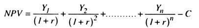
The yields and the cost of capital goods are taken as given. Hence, given the rate of discount or interest, we can determine the NPV from the above formula.

On the basis of this criterion a project will be acceptable if its NPV is positive. If the NPV of a project is negative, it would be rejected. The firm can rank projects on the basis of their NPV. If the supply of capital is unlimited the firm will invest in all projects having a positive NPV. However, if the investment capital is limited the firm will invest in the projects having the highest NPV until its funds are exhausted. In Fig. 13.10 we plot NPV on the vertical axis and real investment on the horizontal axis.

Now let us suppose the rate of interest is constant at r₀. At this rate of interest the NPV of different units of capital are calculated and have been ranked value of NPV. The NPV curve is V₀I₀ when the rate of interest is r₀. If the firm has enough funds it will invest up to l₀ where the NPV of the marginal project is zero.

Hence we can say that, investment will be Ol₀ when the rate of interest is r₀. If the rate of interest increases to r₁, the NPV for each project will be lower than before, provided the supply price and yields remain unchanged. This means that the NPV curve will shift downward when the interest rate increases and the NPV curve becomes V₁I₁. This shows that at a higher rate of interest investment will be lower and hence there is an inverse relationship between the rate of interest and the level of investment. The investment function can thus be written as I = l(r) such that I’(r) < 0.

Expectations:

The MEC is calculated on the basis of yields which can be obtained from the life-time of the machine. These yields are expected but not actual. These expected yields require the expected variable costs which are associated with the production of this output and the expected future price levels.

Thus, expectations enter into the determination of the level of investment. But the expectations may or may not be fulfilled. There is no certainty that the expected yields required in the calculation of the MEC will materialize in practice. Expectations are uncertain and also volatile. They may change drastically in response to the general mood of the business community, news of technical developments, political events, rumors, etc.

One source of uncertainty is the possibility that a machine may become technologically obsolete sooner than expected. For this reason firms may often consider the ‘pay-out period^– for a new plant, rather than its life span. The pay-out period is the period of recovering the cost of the plant.

The firms normally calculate the rate of yield by fixing the pay-out period. If the firm takes a pay-out period of five years, it implies a rate of 20% yield of the cost of the plant. If the firm is not sure that it can achieve this return it will not undertake the investment,

It is true that some machines may have a fairly short expectation of life which may, in fact, be two or three years but not ten of fifteen years. This reduces uncertainty. When uncertainty is less investment will be more interest-elastic.

The problem of uncertainty may be tackled in two ways. One is to consider a frequency distribution of possible yields of any year with the corresponding probabilities. The weighted arithmetical mean of these yields may be taken as the most probable yield of that year. Another way is to consider the “certainty equivalent” of uncertain values which is the objective value of the distribution, plus any premium or less any discount for uncertainty.

Capacity of the Capital Goods Sector:

Gross investment means addition to the stock of capital. Investment takes place when firms are not in equilibrium or optimum. If a firm has less than optimum capital, and if the capital goods are available, then investment can take place very rapidly. However, if capital goods are in short supply, then the rate of investment will be determined by the production capacity of the capital goods industries.

Now, suppose that a firm is in optimum capital stock. No investment will take place unless interest rate falls. If, however, the interest rate falls, the optimum stock of capital will increase and the rate of investment for a single firm will depend on the capacity of the Capital Goods Sector.

For the economy as a whole the gross investment will also depend on the production capacity of the Capital Goods Industry. Net investment will also depend on the capacity of capital goods industries less the annual rate of depreciation.

In the present analysis three rates of investment are possible. It the optimum stock of capital is greater than the actual stock, the firms demand more capital and the capital goods industries will operate at full capacity to meet gross investment need and net investment will be equal to gross investment minus depreciation.

If the optimum stock of capital does not grow at the same rate as the actual stock, the actual stock will be equal to the optimum stock and net investment will be zero. The third rate of investment will occur when the optimum stock falls short of actual stock. In that case, net investment will be negative, at a rate determined by the rate of depreciation.

This analysis has an important implication in that the capital goods industries oscillate violently between conditions of feverish activity and stag­nation. When the industry, in general, is short of capital, capital goods industries are operating at full capacity and it is trying to expand its own capacity. Thus, the capital goods industry’s effort to add its capacity extends and intensifies the boom.

In depression, capital goods industry itself had excess capacity and it will prolong depression. From this analysis we can conclude that, if we start from an equilibrium position and if the optimum stock increases, a boom of considerable consequence may follow. On the other hand, when the actual is greater than optimum, gross investment is zero, capital goods industry stops producing and depression spreads in the whole economy.

Accelerator Theory of Investment:

Now we like to discuss the ‘accelerator’ theory of investment. According to this theory, the level of current net investment depends on past income changes.

In its simplest form, this can be written as follows:

I_t = v(Y_t – Y_{t – 1}), where I_t is net investment in current period, Y_t is the current national income, Y_{t – 1} is national income in the previous period, v is an ‘accelerator’, a constant. Gross investment is equal to net investment plus any replacement investment. So we can write: GI = v (Y_t –Y_{t – 1}) + R_t, where GI is current gross investment and R, is current replacement investment.

For the accelerator theory to be valid, it is necessary that firms must demand additional capital to meet the increased demand for their product. Consider the following example.

Let us assume that, a single firm which initially has a stock of ten machines each of which is capable of producing 50 units of output per year. To keep the analysis simple, assume that, there is no depreciation so that, there is no need to think about replacement investment.

Suppose initially the total demand for the firm’s product is 500 units. This is shown for year 1 in Table 1: note that, the desired capital stock to meet this demand is ten machines and since the firm already has ten machines, no net investment is necessary.

So long as demand stay at 500 units, no net investment will be necessary. Now, suppose in year 2, demand increases to 1,000 units — the desired capital stock will rise to 20 machines and to achieve this, net investment of ten machines is necessary. In year 3, demand has risen to 1,500 units, so that, the desired capital stock goes up to 30 machines— since the firm has already 20 machines, another 10 need to be added. Note that, although demand has risen in year 3, net investment has remained the same.

In year 4, demand continues to increase by 250 units to 1,750 units: the desired capital stock goes up to 35 and so net investment of 5 machines is necessary. Since demand has risen by a small amount than previously, investment has actually fallen. In year 5, demand is still 1,750 units — the firm has already 35 machines necessary to meet this demand and so no new machine (investment) is required.

The example highlights the following points about the theory:

(a) To maintain net investment at a constant positive level, demand for the firm’s product must rise at a steady rate.

(b) For net investment to increase, demand must be increasing at an increasing rate.

(c) If demand should level off and remain constant, net investment will fall to zero.

Note that, the relationship expressed in Table 1 can be written as follows : NI = 1/50 (D_t – D_{t – 1}) where NI is the net investment of the firm, D_t is the current demand for the firm’s product and D_{t – 1} is last year’s demand for the firms product. If all firms behave in a similar way to this, then we can say that, the aggregate net investment in the economy will depend on changes in aggregate demand — they have to be measured in value terms and since the value of aggregate demand in equilibrium is the same as national income, we have I_t = v(Y_t – Y_{t – 1}) .

Two main criticisms may be advanced against this theory:

(1) It assumes that, firms faced with increased demand for their products will immediately attempt to increase their capital stock. This means that there is no excess capacity. This is unrealistic — it is more likely that firms would be able to meet initial increase in demand by allowing excess capacity that it already there.

(2) It fails to take into consideration businessmen’s expectation. If business­men consider the increase in demand to be temporary, they would not respond to it at all: this is likely to be the case if they are generally pessimistic about the future. Alternatively, if they are generally optimistic and see the increase in demand as a signal for further increases, they may buy more machines than predicted by the theory.

In conclusion, we can say that, net investment in an economy will depend on the following factors:

(1) The rate of interest (r);

(2) National income changes in the past;

(3) The state of business expectation (B). We can write the function as: I_t = f (r, Y_t – Y_{t – 1}, B).

However, since it takes time for firms to adjust their capital stock in response to changes in demand, it may be realistic to introduce a time lag into the function and write: I_t =f(r, Y_{t – 1} – Y_{t -2}, B). Only empirical analysis can tell which of the three variables is the most important.