Price and Demand for a Good | Economy

In this article we will discuss about the relation between the price and demand for a good in an economy.

1. Price-Demand Relation for a Non-Inferior (Normal or Superior) Good:

As it is know, M and p_Y remaining constant, if p_x diminishes (increases), then good X becomes relatively cheaper (dearer) and so the consumer buys more (less) of good X owing to the SE. If X is not an inferior good to the consumer, then owing to the IE of the fall (rise) in p_x, he would buy the same quantity or more (less) of good X.

Therefore, if the good X is non-inferior, i.e., if it is normal or superior, then owing to the price effect, or, the total effect (= SE + IE) of a change in the price of X, the quantity demanded of X increases, or, decreases according as its price diminishes, or, increases.

That is, it may be said that in the case of a normal or a superior good, the law of demand would be effective. The matter can be explained with the help of Fig. 6.27 (a).

Here good X (and, also, good Y) has been supposed to be normal or superior, i.e., non- inferior.

Rremember that if the income effect of a fall in p_x is zero, then also good X is considered to be a normal (i.e., non-inferior) good. This case can be illustrated with the help of Fig. 6.27(c). In this figure, initially, the budget line and the equilibrium point of the consumer are, respectively, L₁M₁ and E₁ (x₁, y₁) on IC₁.

Now suppose, the price of good X (p_x) diminishes, the money income of the consumer and the price of good Y (p_Y) remaining unchanged. As a result, the budget line would rotate from L₁M₁ to L₂M₂ and the consumer’s equilibrium point would move from E₁ (x₁, y₁) on IC₁ to E₂ (x₂, y₂) on a higher IC, viz., IC₂. This movement from E₁ to E₂,  represents the price effect (PE) of the said fall in p_x.

The substitution effect (SE) can be obtained with the help of compensating variation in income (CVI), Owing to CVI, the consumer’s budget line would have-a parallel leftward shift from L₁M₂ to ST, and his equilibrium would move from point E₁ (x₁, y₁) to point E₃ (x₃, y₃) along the same IC, i.e., IC₁. The movement in his equilibrium point from E₁ to E₃ represents the SE.

Owing to this effect, the consumer purchases more of X (= x₃ > x₁) and less of Y (= y₃ < y₁), X being relatively cheaper now and Y being relatively dearer. After isolating this SE in PE, the consumer  may be given back the amount of money that was taken away from him by way of CVI.

As this is done, his budget line would have a reverse parallel shift from ST to L₁M₂, and his equilibrium point would move from E₃ (x₃, y₃) to E₂ (x₂, y₂). This movement in his equilibrium point from E₃ on IC₁ to E₂ on IC₂ represents the IE. Since the movement from E₃ to E₂ is a vertical movement, the IE of the said fall in p_x upon the purchase of X has been zero here, i.e., here 

PE = SE + IE = SE + O = SE.

That is, here, the price effect of a fall in p_x upon the purchase of X has coincided with the substitution effect.

2. Price-Demand Relation in the Case of an Inferior Good:

In order to ascertain the price-demand relation for an inferior good, keep in mind the nature of the SE and IE for such a good. For, the sum total of SE and IE is the price-effect which actually underlines the price-demand relation for a good.

As regards the SE, remember that the nature of the SE is the same for an inferior good as for a non- inferior good. Other things remaining the same, if only the price of a good decreases (or increases), then, owing to the SE, the consumer will increase (or decrease) the quantity purchased of the good, since the good has now become relatively cheaper (or dearer).

However, the nature of the IE is not the same for all the goods. If the price of a good, ceteris paribus, decreases (or increases), then consequently the real income of the consumer will increase (or decrease), and, owing to the income effect, the consumer will decrease (or increase) the purchase of the good if it is an inferior good, and he will increase (or decrease) the purchase of the good if it is a normal or a superior good.

Keeping in mind these points about the nature of the SE and IE, it may now be derived that the price- demand relation for an inferior good. It shall be assumed here that, of the two goods, X and Y, that the consumer buys, X is an inferior good.

The price-demand relation of an inferior good (X) may be of the following three types depending on the degree of inferiority of the good to the consumer:

(I) In the event of p_x decreasing (or increasing), the income effect fall (or rise) in the demand for X may be less than the substitution effect rise (or fall) in its demand.

In this case, the price-demand relation for the inferior good, X, will be inverse, i.e. if p_x decreases (or increases), then owing to the price effect (= IE + SE), the demand for X would rise (or fall). Therefore, in this case, the law of demand will be effective. That is, the consumer’s individual demand curve for good X will be negatively sloped like the curve dd in Fig. 6.28(a).

(II) In the event of p_x decreasing (or increasing), the income effect fall (or rise) in demand for X may be equal to the substitution effect rise (or fall) in its demand.

In this case, the price effect (= IE + SE) would be equal to zero. Therefore, the consumer’s demand for good X would remain unchanged even if there is change in its price. That is, in this case, the law of demand will not be effective. The consumer’s demand curve for X in this case will be a vertical straight line like dd in Fig. 6.28(b).

(III) In the event of p_x decreasing (or increasing), the income effect fall (or rise) in demand for X may be greater than the substitution effect rise (or fall) in its demand.

In this case, the price-demand relation for the inferior good, X, will be positive, i.e., if p_x decreases (or increases), then owing to the price effect (= IE + SE), the demand for X will also fall (or rise). Therefore, in this case, the law of demand will not be effective.

The demand curve of the consumer for the inferior good X will be positively sloped like the curve dd in Fig. 6.28 (c). The (inferior) goods, for which the demand curve is obtained to be positively sloped, are called the Giffen goods after Sir Robert Giffen (1837-1910), an Irish economist.

In the analysis,three types of price-demand relation for an inferior good (here X) is obtained depending on the degree of its inferiority to the consumer. Of these three cases, the degree of inferiority of good X is the least in case (I). In this case, the magnitude of the IE fall (or rise) in demand for X as p_x falls (or rises), has been smaller than the SE rise (or fall) in demand, and the law of demand is able to operate.

On the other hand, the degree of inferiority of good X is the highest in case (III). In this case, the magnitude of the IE fall (or rise) in demand for X as p_x falls (or rises), has been larger than the SE rise (or fall) in demand, and the law of demand cannot operate.

Finally, the degree of inferiority of good X in case (II) is a midway between cases (I) and (III). Here the magnitude of the IE fall (or rise) and that of the SE rise (or fall) in demand for X have been equal and the price effect has been obtained to be zero. Therefore, the law of demand is ineffective in this case.

3. Geometrical Illustrations of Price-Demand Relation for an Inferior Good:

Now let’s explain the type (I) of price-demand relation for an inferior good that is discussed with the help of Fig. 6.29. The consumer is buying the goods X and Y. Good X of these two, is an inferior good. In Fig. 6.29, initially, the consumer’s budget line is L₁M₁ and his equilibrium point is E₁ (x₁ y₁) on the indifference curve IC₁.

Now suppose, the money income of the consumer (M) and the price of good Y (p_Y) remaining unchanged, the price of good X (p_x) has diminished.

As a consequence, the budget line of the consumer, L₁M₁, rotates anticlockwise about the point L₁ to the position of, say, L₁M₂, and his equilibrium point moves from E₁ on IC₁ to E₂ on a higher IC, IC₂. The consumer moves on to a higher IC because his real income has increased.

The movement in consumer’s equilibrium point from E₁ to E₂ represents the price effect. Owing to this effect, the consumer purchases x̅₁x̅₂ more of good X. Therefore, here, the price-demand relation for the inferior good X has been negative, i.e., here the law of demand is effective.

Now break up the PE into an SE and an IE, it is found that, as a consequence of the ceteris paribus fall in p_x, the demand for X has increased by x̅₁x̅₃ because of SE and decreased by x̅₃x̅₂ because of IE. Since x̅₁x̅₃ > x̅₃x̅₂ in Fig. 6.29, the consumer’s demand for good X has increased (by x̅₁x̅₃ – x̅₃x̅₂ = x̅₁x̅₂) as a result of the fall in p_x.

Therefore, here the demand for the inferior good (X) will increase when its price falls. That is, although good X is an inferior good, it would be subject to the law of demand. The consumer’s demand curve for good X in this case would be sloping downwards towards right [Fig. 6.28(a)].

Now let’s explain the type (II) of price-demand relation for an inferior good with the help of Fig. 6.30. In this figure, initially, the consumer’s budget line and his equilibrium point have been L₁M₁ and E₁ respectively.

At the point E₁ on IC₁, the consumer buys x₁ of the inferior good, X. Now, as a consequence of a ceteris paribus fall in p_x, the consumer’s budget line and his equilibrium point have been L₁M₂ and E₂ respectively.

The point E₂ lies on a higher IC, viz., IC₂, since the real income of the consumer has increased. Now since the point E₂ lies just to the north of the point E₁ the consumer’s purchase of good X owing to the price effect has not changed at all—it remains unchanged at x = x₁ = x₂. Here, the movement in the equilibrium point of the consumer from E₁ to E₂ represents the price- effect, which is zero upon the purchase of X.

In Fig. 6.30, it is found that as a consequence of the ceteris paribus fall in p_x, the consumer’s purchase of good X has increased by x̅₁x̅₃ because of the SE and decreased by x̅₃x̅₁ because of the IE. Since the magnitude of the SE-rise and that of the IE-fall in the purchase of good X have been equal, the price effect (= SE + IE) in this case has been equal to zero.

That is, the fall in p_x here would have no effect on the demand for X. In a similar way it can be seen that a rise in p_x in this case also would have no effect on the demand for X. Therefore, the law of demand would not be effective here. The consumer’s demand curve for good X would be a vertical straight line in this case [Fig. 6.28(b)].

Finally, the type (III) price-demand relation for the inferior good X can be explained with the help of Fig. 6.31. In this figure, it is also assumed that initially, the budget line of the consumer and his equilibrium point are L₁M₁ and E₁ on IC₁.

Now, as a consequence of the ceteris paribus fall in p_x, the consumer’s budget line and his equilibrium point would be L₁M₂ and E₂ on a higher IC, viz., IC₂. The movement in the consumer’s equilibrium point from E₁(x₁, y₁) to E₂(x₂, y₂) represents the price effect in this case. Because of this effect the consumer buys xjx₂ less of X₁.

Now break up this PE into an SE and an IE,it may be found in Fig. 6.31 that, as a consequence of the fall in p_x, the consumer’s purchase of X has increased by x̅₁x̅₃ because of SE and decreased by x̅₃x̅₂ because of IE.

Since x̅₁x̅₃ < x̅₃x̅₂ in Fig. 6.31, the consumer’s demand for good X has decreased in this case by x̅₃x̅₂ -x̅₁x̅₃ = x̅₁x̅₂ as a result of the fall in p_x. Therefore, here the demand for the inferior good, X, will decrease when its price falls. That is, the price-demand relation for the inferior good X has been positive in this case.

The consumer’s demand curve here would be sloping upward towards right [Fig. 6.28(c)]. The inferior good in this type (III) case is called a Giffen good. It may be also noted that the type (III) case is known as Giffen Paradox.

It has been discussed that the three types of price-demand relation that might exist for an inferior good. these cases can be explaines with the help of Figs. 6.29-6.31. In all these three figures, the consumer has moved from the point E₃ to E₂ owing to the income effect.

Therefore, the lines joining the points E₃ and E₂ in these figures are the ICCs. Since good X is an inferior good, the ICCs in all the three figures have bent towards the y-axis. Here, it may be observed that the higher the degree of inferiority of good X to the consumer, the more prominently the ICC would bend towards the y-axis.

4. Demand Curve from the Price-Consumption Curve:

Now see how the demand curve of a consumer for a particular good can be obtained from his price-consumption curve (PCC) for the good. Here, it ay be assumed that of the two goods that the consumer uses, one is good X and the other good is money, the quantity of which may be denoted by y.

In Fig. 6.32, the quantity of good X (i.e. x) is measured which is used by the consumer, along the horizontal (x-) axis, and the quantity of money retained by the consumer for himself along the vertical (y-) axis.

Here suppose, the consumer has OL₁ of money with him and initially, the price of X (p_x) is such that if he spends all this money on X, he would be able to buy OM₁ of X. That is, in the initial situation, the budget line of the consumer is L₁M₁ and the price of X is OL₁/OM₁ which, is the numerical value of the slope of the budget line.

Again, initially, the equilibrium point of the consumer is E₁ which is the point of tangency between the budget line and one of the consumer’s ICs, viz., IC₁. At E₁, the consumer is buying OA₁ of good X.

Now, other things remaining the same, if p_x diminishes, the consumer’s budget line would rotate anticlockwise about the point L, and it would now become a line like L₁M₂. p_x now has diminished from OL₁/OM₁to OL₁/OM₂ (which is the numerical slope of the line L₁M₂). Now, the consumer’s equilibrium point would be the point of tangency E₂ between the budget line L₁M₂ and the indifference curve IC₂.

At E₂, the consumer would purchase OA₂ of good X (OA₂ > OA)). If p_x diminishes again, then the consumer’s budget line would become a line like L₁M₃ and he would be in equilibrium at the point E₃ on an IC like IC₃. At E₃, the consumer would buy OA₃ of good X at the price of OL₁/OM₃. Now, as known that the curve passing through the points E₁, E₂, E₃,. . . is the consumer’s PCC for good X.

The point L₁ is also a point on this curve. Let’s now see how the consumer’s demand curve for good X from his PCC for the said good may be obtained. In order to obtain this curve, draw the lines B ₁F₁, B₂F₂, and B₃F₃ as parallel to the lines L₁M₁, L₁M₂ and L₁M₃ respectively.

Here it is assumed that A₁B₁ = A₂B₂ = A₃B₃ = one unit of good X. Now when the budget line of the consumer is L₁M₁, p_x = OL₁/OM₁ = A₁F₁/A₁B₁ = A₁F₁ (^._.^.L₁M₁ΙΙ B₁F₁ and A₁B₁ =1). Similarly, when the budget line of the consumer is L₁M₂ and L₁M₃, p_x to be equal to A₂F₂ and A₃F₃, respectively.

Therefore, in Fig. 6.32, when the price of good X is A₁F₁, A₂F₂ and A₃F₃, his purchase of X would be OA₁, OA₂ and OA₃ respectively. That is, the points F₁, F₂ and F₃ would be the points on the consumer’s demand curve for X, and this curve would be obtained by joining these points. This curve is dd in Fig. 6.32.

So far as have been discussed how the consumer’s demand curve for good X can be derived from his price-consumption curve. In Fig. 6.32, the PCC curve is moving downward towards right initially, then it is sloping upward towards right.

This gives us that as the price of good X diminishes, the consumer always buys more of the good, i.e., here the law of demand is effective. That is why the demand curve for good X (dd) that have obtained is sloping downward towards right.

5. Inferior Good and Giffen Good:

On the basis of our discussion of the price-demand relation for an inferior good, it may be said that all Giffen goods are inferior goods but all inferior goods are not Giffen goods. In other words,  a Giffen good must be an inferior good, but an inferior good may not be a Giffen good.

By definition, owing to the price effect (PE = SE + IE) of a ceteris paribus fall in the price of a Giffen good, X, the consumer’s demand for the good diminishes. But, because of the substitution effect (SE) of the said fall in p_x, the consumer’s purchase of X must increase, since X is now relatively cheaper.

Therefore, the fall in demand for X as p_x diminishes, can be obtained, only when the IE of the fall in p_x reduces the demand for good X, and by a magnitude greater than that of the SE rise in demand for X, i.e., only when X is an inferior good. This gives us that a Giffen good must be an inferior good.

The point can be explained with the help of Fig. 6.31. Here, because of the SE of the fall in p_x, consumer’s demand for X has increased by x̅₁x̅₃.

If good X is a Giffen good then its demand would fall because of the income effect (of a rise in real income) due to the fall in p_x and demand would have to fall by a greater magnitude than that of x̅₁x̅₃. In Fig. 6.31, the decrease in demand due to the IE has been by x̅₃x̅₂ (> x̅₁x̅₃). Therefore, if X is a Giffen good, then it must be an inferior good.

On the other hand, if X is an inferior good, then because of the IE of a fall in p_x, the demand for the good would decrease and owing to the SE, demand for the good would increase.

Now, if the magnitude of the SE rise in demand for X is greater than that of the IE fall, then the PE (= IE + SE) of the fall in P_x would be a rise in the demand for X, giving us that X here is not a Giffen good. Therefore, it is obtained that if X is an inferior good, then it may not be a Giffen good.

The point can be explained with the help of Fig. 6.29. Here owing to the IE of a fall in p_x, the consumer’s demand for X has fallen by the magnitude of x̅₃x̅₂. Therefore, here X is an inferior good. But owing to the SE of the fall in p_x the demand for X has increased by the magnitude of x₁x₃.

Since x̅₁x̅₃ > x̅₃x̅₂, the PE of the fall in p_x ultimately has been a rise in the demand for X by the magnitude x̅₁x̅₃ – x̅₃x̅₂ = x₁x₂. Therefore, although good X here is an inferior good, it is not a Giffen good.

Lastly, as obtained in Fig. 6.30 that the IE-fall in the demand for an inferior good X by the magnitude x̅₃x̅₁, may be equal to SE-rise in demand by the same magnitude giving us the PE of the said fall in p_x to be equal to a zero change in demand for X, not a fall in demand for X. Therefore, here also, X may be an inferior good, but it will not be a Giffen good.

On the basis of our above discussion, it may be concluded that a Giffen good must be an inferior good, but any inferior good may not be a Giffen good.

6. Demand Curve and Price-Elasticity of Demand:

An individual’s demand curve for a good tells us what would be the change in his demand for the good when the price of the good changes by a certain amount. The elasticity of quantity demanded for a good in response to a change in its price is called the price-elasticity of demand.

More specifically, the percentage change in the quantity demanded of a good in response to a 1 per cent change in its price, is known as the coefficient of price-elasticity of demand (E_P). For example, if as a result of a 1 percent increase in the price of the good, the individual buys 2 per cent less of the good, then E_P = −2. The formula for obtaining E_P at any particular price-quantity combination of the good is

From the definition of price elasticity of demand for a commodity for a particular individual it is obtained that E_p is defined at a point on his demand curve for the good. Let us suppose that the individual’s demand curve for the good is dd in s. 6.33. At any point, A, on this curve, when the price of the good is p (or OP), the individual buys the quantity q (or OQ) of the good.

Therefore, at the point A(p,q),

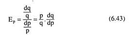
Here dp is an infinitesimally small change in the price of the good and dq is the resulting change in the quantity purchased of the good, and dq/dp is the reciprocal of the slope of the demand curve at the point A (since, the slope of the demand curve is dp/dq). Remember here that if the law of demand operates (i.e., if dq ≠ 0 when dp ≠ 0), E_p would be negative (E_p < 0).

On the other hand, if the law of demand is not effective (i.e., if dq = 0 when dp ≠ 0, or dq ≠ 0 when dp ≠ 0), E_p = 0 or E_p > 0, i.e., in the case of an exception to the law of demand, E_p ≥ 0.

7. Relation between the Price-Consumption Curve and Price-Elasticity of Demand:

There is a close relation between the price-consumption curve (PCC) and the price-elasticity of demand for a good. Remember here that the coefficient of price-elasticity of demand (E_p) would be negative because of the law of demand, and the absolute or the numerical value (e) of this coefficient would be

……………(6.44)

The relation between PCC and e is discussed with the help of Fig. 6.34. Here it is assumed that, of the two goods that the consumer uses, one is good X (measured along the horizontal axis), and the other is money (measured y along the vertical axis). The indifference curves (ICs) of the consumer are given in the figure.

The PCC of the consumer for changes in the price of good X is also given. It is assumed here that the consumer has OL, amount of money with him. Let us suppose that, initially, the budget line of the consumer is L₁M₁ i.e., the price of good X is such that if the consumer spends all his money (OL,) on X, he would be able to buy OM, of the good.

In Fig. 6.34, the consumer’s initial equilibrium point is the point of tangency E, between his budget line L₁M₁ and one of his ICs, viz., IC₁. At E₁, the consumer buys OA) of good X and he would retain OP of money with him, and so he would spend L₁P of money to buy OA, of X.

It is obvious from Fig. 6.34 that if the price of good X (p_x) diminishes ceteris paribus his budget line would rotate from L₁M₁ to a line like L₁M₂ and his equilibrium would move along the negatively sloped portion of his PCC from E₁ on IC₁ to E₂ on IC₂.

As a consequence of this, his purchase of good X would rise from OA, to OA₂, and the amount of money retained by him would diminish from OP to OQ, and so the amount of money spent on X would increase from L₁P to L₁Q. That is, as p_x has diminished, the consumer has increased his expenditure on X.

Therefore, here the percentage rise in his demand for X has been greater than the percentage fall in p_x, i.e., from eq(6.44) e > 1. In other words, along the negatively sloped segment of the PCC, e > 1.

It is also seen in Fig. 6.34 that if p_x falls further, and as a consequence, the consumer’s budget line rotates from L₁M₂ to L₁M₃, his equilibrium point would move along the horizontal portion of his PCC from E₂ to E₃.

As a result, the consumer’s purchase of X would increase from OA₂ to OA₃ and the amount of money he would retain would remain the same at OQ (since PCC has been horizon­tal), and so his expenditure on X would also remain the same at L₁Q.

That is, here, as p_x has diminished and demand for X has increased, the consumer has kept his expenditure on X unchanged. Therefore, here, the percentage rise in his demand for X has been equal to the percentage fall in p_x, giving us e = 1. In other words, along the horizontal segment of the PCC, e = 1.

Lastly, as seen in Fig. 6.34, if the consumer’s budget line becomes L₁M₄ as a consequence of a still further fall in p_x, his equilibrium point would move from point E₃ to point E₄ along the upward (positively) sloping portion of his PCC. The consumer now would demand more of X, his purchase would rise from OA₃ to OA4, and his expenditure on good X would also fall from L₁Q to L₁R.

That is, here as p_x has fallen, the consumer’s expenditure on X has also fallen giving e < 1 [from eq(6.44)]. Therefore, along the positively sloped portion of the PCC, e < 1.

On the basis of the analysis, it may said that along the negatively sloped segment of the PCC of a consumer for a certain good, e would be greater than one (e > 1), along the horizontal segment, e would be equal to one (e = 1), and lastly, along the positively sloped segment of the PCC, e would be less than one (e < 1). Thus, it can be read about the price-elasticity of a consumer’s demand for a good from the PCC.