Short Run Cost of a Firm | Microeconomics

In this article we will discuss about:- 1. Total Fixed Cost, Total Variable Cost and Short Run Total Cost 2. TVC Curve of the Firm 3. Total Fixed Cost (TFC) Curve 4. Short Run Total Cost Curve of the Firm 5. Average Fixed Cost and Average Fixed Cost Curve 6. Average Variable Cost and the Average Variable Cost Curve and Others.

Total Fixed Cost, Total Variable Cost and Short Run Total Cost:

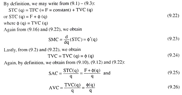
In the short run, to produce a particular quantity of output per day, the cost that the firm has to incur for the fixed inputs is called the total fixed cost (TFC) per day, and the cost that it has to incur for the variable inputs is called the total variable cost (TVC) per day.

The sum total of TFC and TVC at any particular quantity of output (q) is called the short-run total cost (STC) per period. Therefore, we may write, at any particular q,

STC = TFC + TVC                                     (9.1)

We have to remember here that, in the short run, as q changes (increases or decreases), the quantities used of the variable inputs and TVC would also change (increase or decrease). But, in spite of changes in q, the quantities of the fixed inputs and TFC would remain unchanged.

That is, we obtain:

TVC Curve of the Firm:

We shall assume here that the firm uses two variable inputs X and Y along with some fixed inputs and produces an output Q. Its short-run production function is given by (8.1):

q = f(x,y) [(8.1)]

The (short-run) TVC function (9.2) of the firm is obtained from its short-run production function (8.1), given the prices of the variable inputs. This function gives us the functional relationship between the firm’s quantity of output produced (q) and its TVC.

Let us again write below this function:

TVC = TVC (q); d(TVC)/dq > 0 [eqn. (9.2)]

Let us now see how the firm’s TVC function may be derived from its production function, given the prices of the inputs. As we know , the isoquants (IQs) of the firm may be obtained from its production function (8.1) or (8.21).

Also, the firm’s iso-cost lines (ICLs) are obtained from the given prices of the variable inputs, r_x and r_Y, and the proposed TVC, viz., TVC₁, TVC₂, TVC₃,…. We obtain, then, the expansion path of the firm as the curve joining the point of origin ‘O’ and the points of tangency between the IQs and the ICLs . We shall now see that the firm’s TVC function or, the TVC curve can be obtained directly from its expansion path.

We may explain this with the help of Fig. 9.1. Here three of the firm’s IQs have been given as IQ₁, IQ₂ and IQ₃. Let us suppose these IQs represent the output levels of q₁, q₂ and q₃ respectively. Again, three of the firm’s ICLs here are L₁M₁, L₂M₂ and L₃M₃.

We have assumed that the ICLs represent TVC levels of TVC₁, TVC₂ and TVC₃, respectively. In Fig. 9.1, the curve OK is the expansion path of the firm. Each point on this path is a point of tangency between an IQ and an ICL of the firm. For example, the point E) on this path is the point of tangency between IQ₁ and an ICL, viz., L₁M₁.

From the expansion path, we can see that if the firm intends to produce a particular quantity q₁ of output, then it would have to remain at the point E₁ (x₁, y₁) in Fig. 9.1. Since E) is the point of tangency between IQ₁ (for q = q₁) and an ICL, L₁M₁ (for cost level TVC₁), we also have, TVC₁ is the minimum TVC at q = q₁ where TVC₁ = r_x.x₁ + r_Y.y₁.

Therefore, the point E₁ on the expansion path implicitly gives us the combination (q₂,TVC₁) of the quantity of output produced and its minimum TVC, although explicitly the point gives us the combination (x₁.y₁) of the variable input quantities. Just like E₁, the points E₂ and E₃, on the expansion path, would implicitly give us the combinations (q₂, TVC₂) and (q₃, TVC₃).

Now, if we plot the combinations (q₁, TVC₁), (q₂, TVC₂) and (q₃, TVC₃) as the points R₁, R₂ and R₃ in a separate diagram like Fig. 9.2, then the curve joining the origin O and these points would give us the TVC curve or the TVC function of the firm.

The point of origin ‘O’ would be a point on the TVC curve, because, at q = 0, the quantities used of the variable inputs would be reduced to zero and the TVC of the firm would become equal to zero. The TVC curve of the firm gives us its TVC at any particular q.

Therefore, how the TVC curve of the firm has been obtained in Fig. 9.2 from its expansion path given in Fig. 9.1. The expansion path, again, is obtained from the firm’s short-run production function as given by its IQs, given the prices of the variable inputs. In other words, the firm’s TVC can be derived from its short-run production function and the prices of the variable inputs.

There is a one-to-one correspondence between the points on the expansion path and those on the TVC. For example, for the points E₁, E₂ and E₃ on the expansion path, we have the points R₁, R₂ and R₃, respectively, on the TVC curve of the firm.

We may also note that q may rise in the short run only when more of the variable inputs are used. That is why the TVC curve of the firm would be positively sloped or upward rising—as q rises, TVC would rise.

Lastly, it should be remembered that the TVC curve gives us the minimum possible cost for the variable inputs at any q, since a point on the TVC curve is nothing but the transformation of a point tangency (least cost point) on the expansion path.

Properties of the Total Variable Cost (TVC) Curve:

The shape of the TVC curve of the firm would be like that of the TVC curve given in Fig. 9.2.

The properties of this curve are:

(i) The TVC curve would be sloping upward towards right or it would be a positively sloped curve. This is because it is assumed in the production theory that the prices of the variable inputs remain unchanged and, in the short run, the firm can increase its production only by increasing the quantities used of the variable inputs. Therefore, as output increases, the firm’s TVC also increases, giving us the positive slope of the TVC curve.

(ii) The TVC curve starts from the point of origin. Because, in the short run, if the quantity produced (q) is reduced to zero, the use of the variable inputs can also be reduced to zero, giving us TVC = 0.

(iii) Initially, the TVC curve is concave downwards and then it is convex downwards. That is, the TVC curve is a third degree curve. The general form of such a curve is

C = aq³ + bq² + cq + d (9.5)

where q is the quantity of output and C is the cost term. Since, because of property (ii), TVC = 0 when q = 0, we would not have any constant term like ‘d’ of (9.5) in the equation of the TVC curve:

TVC = aq³ + bq² + cq (9.6)

This concave-convex property [property (iii)] of the TVC curve is obtained from the convex- concave property of the total product curve of a variable input, say, labour.

This total product curve is like the TP_L curve given in Fig. 8.1. Again since the said property of the TP_L curve reflects the law of variable proportions (LVP), the property (iii) of the TVC curve or the concave- convex shape of the curve also reflects the features of the LVP.

  

Correspondence between the Convex-Concave Shape of the Total Product Curve of a Variable Input and the Concave-Convex Shape of the Total Variable Cost Curve:

In the discussion of the LVP, we generally assume that the firm uses only one variable input, labour, to produce its output. On the other hand, the TVC curve is obtained on the basis of the isoquants (IQs) and iso-cost lines (ICLs), and the expansion path of the firm, where it is assumed that the firm uses two variable inputs (X and Y) along with some fixed inputs.

Now, to measure the quantities of two different variable inputs along one axis and the quantity of output along the other axis, we may very well use the costs for the variable inputs, i.e., TVC, as the index of the quantities used of the variable inputs. This is because, if the quantities used of the variable inputs increase or decrease, their prices remaining unchanged, then the TVC would also increase or decrease.

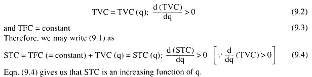
Following the TP_L curve of Fig 8.1, we have constructed the total product curve of the variable inputs (here X and Y) in Fig. 9.3(a) and we have named this curve TP_V. From the TP_V curve we would know what the total product (q) would be at any TVC which is the index of the quantities used of the variable inputs (X and Y).

In Fig. 9.3(a), we have shown the TP_V curve. Its shape would be the same as that of the TP_L curve because of the LVP (Fig. 8.1). We have not shown, however, the negatively sloped portion of the TP_V curve, because this portion of the TP curve of any variable input(s) would be irrelevant for a profit- maximising firm’s decision-making.

This is so because, along this portion, as the quantity used of the variable input(s) or TVC increases, TP or the total product (q) of the firm decreases.

Now, along the upward sloping and convex downward portion of the TP_V curve in Fig. 9.3(a), as TVC (i.e., variable input quantities) increases over the interval (0, TVC₀), q also increases, and at an increasing rate over the interval (0, q₀), i.e., over these intervals, as q increases, TVC increases at a diminishing rate.

That is why, in Fig. 9.3(b), we obtain the TVC curve to be upward sloping and concave downwards over the said intervals.

Again, along the upward sloping and concave downward portion of the TP_V curve in Fig. 9.3(a), as TVC increases over the interval (TVC₀, TVC₁), q increases at a diminishing rate over the interval (q₀, q₁), i.e., as q increases, TVC increases at an increasing rate over these intervals. That is why, in Fig. 9.3(b), the TVC curve is obtained to be upward sloping and convex downwards over these intervals.

In the above analysis, the concave-convex shape of the TVC curve is obtained from the convex-concave shape of the total product curve (TP_V curve) of the variable inputs. Actually, the concave portion of the TVC curve corresponds to the convex portion of the TP_V curve and the convex portion of the TVC curve corresponds to the concave portion of the TP_V curve.

Lastly, we may note that in Fig. 9.3(a), when q = q₀ (and TVC = TVC₀), the rate of increase of total product of the variable inputs (TP_V or q) w.r.t. variable input quantities, i.e., the marginal product of the variable inputs, as it is called, has increased to its maximum.

For, the E₀ (TVC₀, q₀) point is the last point of convex downward portion of the TP_V curve (before it takes a turn to be concave downwards)—this point is called the point of inflexion of the TP_V curve. Again, in Fig. 9.3(b) when q = q₀ (and TVC = TVC₀), the rate of increase of TVC w.r.t. q [i.e., the marginal cost of production (MC)] has decreased to its minimum.

For, the G₀ (q₀, TVC₀) point is the last point of the concave downward segment of the TVC curve (before it takes a turn to be convex downwards)—this point is the point of inflexion of the TVC curve.

Therefore, the value of q in Fig. 9.3(a), beyond which the TP_V curve becomes concave downwards and the value of q in Fig. 9.3(b), beyond which the TVC curve becomes convex downwards are the same—this value of q is q₀.

Total Fixed Cost (TFC) Curve:

In the short run, the firm’s total fixed cost (TFC) is a constant independent of q [eqn. (9.3)]. Therefore, the TFC curve would be a horizontal straight line at the level of the total fixed cost of the firm, as shown in Fig. 9.3(b). In this Fig. 9.3(b), the firm’s TFC has been assumed to be OF = constant. Therefore, its TFC curve has been a horizontal straight line at the level of OF.

Short Run Total Cost Curve of the Firm:

We may now easily obtain the short-run total cost (STC) curve of the firm on the basis of its TVC and TFC curves. For, by definition, if we add the constant amount of TFC to the firm’s TVC at any q, we obtain its STC at that q [eqn. (9.1)].

Therefore, in Fig. 9.2, at q = q₁ we would obtain the STC to be S₁q₁ by adding the TFC = S₁R₁ = OF to the TVC = R₁q₁. Similarly, at q = q₂ and q₃, the firm’s STC would be S₂q₂ and S₃q₃, respectively. If we join the points F and S₁, S₂, S₃, etc. by a curve we would obtain the firm’s STC curve. This curve would start from the point F on the vertical axis, because, as we know, TVC = 0, when q = 0, giving us

STC|_q=0 =TVC + TFC = 0 + OF

= OF = TFC                                 (9.7)

It may be noted here that the TVC curve of the firm starts from the origin. For, if q reduces to zero, the variable input quantities may be brought down to zero giving us TVC = 0. But the STC curve would not start from the origin, because at q = 0, STC ≠ 0. At q = 0, STC = TFC = OF [Fig. 9.3(b)], So the TFC curve would start from a point on the vertical axis at a height equal to TFC.

In the analysis of short-run cost of a firm, the construction of the STC function or the STC curve of the firm has to be accomplished through several stages. First, on the basis of the short-run production function of the firm and the given variable input prices, we obtain the isoquants (IQs) and the iso-cost lines (ICLs) of the firm.

In the second stage, we obtain the expansion path of the firm from the IQs and ICLs, that is, by joining their points of tangency and the point of origin. In the third stage, we obtain the TVC curve of the firm from its expansion path. In the final stage, we obtain the STC function or curve of the firm by shifting the TVC curve vertically by the constant amount of TFC, that is, by adding the constant TFC to TVC at each q.

Properties of the Short-Run Total Cost Curve:

Most of the properties of the short-run total cost (STC) curve of the firm are similar to those of its total variable cost (TVC) curve.

The properties of the STC curve are:

(i) The STC curve, like the TVC curve, is also upward sloping towards right, i.e., as q rises, STC also rises. For as q rises, TVC rises and so STC = TVC + TFC (= constant) also rises.

(ii) At any quantity of output produced (q), we obtain STC if we add the constant amount of TFC to TVC.

Therefore, at each q, the slope of the STC curve would be the same as that of the TVC curve:

where d/dq (STC) and d/dq (TVC) are the slopes of STC and TVC functions, respectively, at any particular q.

Therefore, the range of q over which the TVC and the STC curves are concave would be the same and the range of q over which the two curves are convex would also be the same. In Fig. 9.3(b), we have constructed the STC curve on the basis of the TVC curve assuming the TFC to be equal to OF.

Here both the STC and the TVC curves have been concave over the range of q from 0 to q₀ and both these curves have been convex for q > q₀. We have to remember that the concave-convex property of the TVC curve, and, therefore, of the STC curve, is obtained because of the law of variable proportions (LVP).

Again, since the slopes of TVC and STC curves are the same at each q, the slopes of both these curves have been minimum at q = q₀ at their respective points of inflexion G₀ and H₀ which are the extreme points on their concave portions.

Therefore, at q = q₀, the (same) rate of increase of both TVC and STC has decreased to its minimum, and beyond q₀, this rate again increases as q increases. This rate is called, the marginal cost (MC). So we may say that at q = q₀ or at the points of inflexion of the two curves, G₀ and H₀, the MC would be minimum.

(iii) The STC curve, unlike the TVC curve, does not start from the point of origin ‘O’ It starts from a point like F in Fig. 9.3(b) on the vertical axis. For at q = 0, TVC is equal to zero, but TFC is not equal to zero, it is a positive constant. In Fig. 9.3, it has been assumed that TFC = OF. Therefore, at q = 0, we have

STC = TVC + TFC

= 0 + TFC = TFC = OF > 0

Therefore, the STC curve would start from the point F in Fig. 9.3(b) on the vertical axis.

(iv) Like the TVC curve, the STC curve also is a concave-convex curve [property (ii)]. Therefore, the STC curve would also be a third degree curve. The general form of the STC curve would be

STC = aq³ + bq² + cq + F                (9.8)

Here, at q = 0, we have STC = F (= TFC).

Average Fixed Cost and Average Fixed Cost Curve:

At any particular quantity of the firm’s output (q), the average fixed cost per unit of output is called simply the average fixed cost (AFC). According to this definition, the AFC is obtained if we divide the TFC by q.

Therefore, we may write:

It is evident from equation (9.9) that AFC depends on the firm’s quantity of output (q); the equation gives us the AFC function—AFC is a function of q. We may know the firm’s AFC at any particular q from (9.9), i.e., we may have the different (q, AFC) combinations.

For example, if TFC = Rs 200, then the different (q, AFC) combinations that may be obtained from (9.9) are (5, 40), (10, 20), (20, 10), (40, 5), etc. If we plot these combinations as points in Fig. 9.4, then the curve joining these points would give us the AFC curve of the firm.

Therefore, equation (9.9) is the equation of the AFC curve. From this equation, it is obvious that, as q increases, the firm’s AFC decreases monotonically. Therefore, the AFC curve would be sloping downward towards right. Again, we obtain from equation (9.9) that at any q or at any point on the AFC curve, q x AFC = TFC = constant. That is why the AFC curve, like the one shown in Fig. 9.4, would be a rectangular hyperbola.

Average Variable Cost and the Average Variable Cost Curve:

At any particular quantity of the firm’s output (q), the average variable cost per unit of output is called simply the average variable cost (AVC). According to this definition, the AVC is obtained if we divide the TVC by q.

Therefore, we may write:

It is evident from equation (9.10) that AVC depends on the firm’s quantity of output (q); the equation gives us the AVC function—the AVC is a function of q. We may know the firm’s AVC at any particular q from (9.10). That is, we obtain the different (q, AVC) combinations from (9.10). If we plot these combinations as points on the (q, AVC) plane of Fig. 9.5, then the curve joining these points would give us the AVC curve of the firm.

Equation (9.11) gives us that, since the TVC curve is a third degree curve, the AVC curve of the firm would be a second degree curve. That is, the firm’s AVC curve would be a U-shaped curve like the one shown in Fig. 9.5.

The concave-convex shape of the TVC curve, i.e., its third-degree shape, is obtained because of the LVP [9.2.4(iii)]. Again, the second-degree shape of the AVC curve is derived from the third degree shape of the TVC curve. Therefore, the U-shape of the AVC curve, like the third degree shape of the TVC curve, is obtained from the LVP.

The Geometric Method:

We may also see how the U-shape or the second degree shape of the AVC curve is obtained from the third degree shape of the TVC curve with the help of geometry given in Fig. 9.6. In Fig. 9.6, the firm’s TVC is R₁q₁ at q = q₁ (or Oq₁). Therefore, here, the firm’s AVC would

The straight line OR₁ is also called the guideline to the TVC curve at q = q₁. Similarly, at q = q₂, q₃ and q₄, the firm’s AVC would be, respectively, the slopes of the guidelines OR₂, OR₃ and OR₄ (the guideline OR₃ has not been shown in the figure).

Now, it is obvious from Fig. 9.6(a) that as the firm’s q increases, the guideline to its concave- convex TVC curve becomes flatter, i.e., the slope of this line which is the firm’s AVC, decreases.

At some q, like q = q₄ in Fig. 9.6, the guideline would become so flat as to touch the TVC curve at the point R₄. Here, at q = q₄, the guideline is the flattest and the AVC is minimum. If the quantity of output (q) of the firm increases beyond q = q₄, the guideline becomes steeper, i.e., its slope increases, and so the firm’s AVC increases.

From the above analysis, what we obtain is that as the firm’s output (q) increases initially, the AVC decreases and, at some q (here at q = q₄), the AVC becomes minimum. If q increases beyond this value, the firm’s AVC also increases.

Therefore, the AVC curve of the firm would be U-shaped. The AVC curve associated with the TVC curve in Fig. 9.6(a) has been shown in Fig. 9.6(b). Here, till q rises to become q = q₄, the AVC curve of the firm has been sloping downward towards right, the AVC curve has reached its minimum at q = q₄, and as q increases beyond q₄, the AVC curve has been upward sloping towards right.

Short-Run Average Cost and the Short-Run Average Cost Curve of the Firm:

At any particular quantity of the firm’s output (q), the average cost of production per unit of output in the short run, is called simply the short-run average cost (SAC) of the firm. The SAC would be obtained if we divide the short-run total cost (STC) of production by q.

We may, write, therefore:

It is obvious from equation (9.12) that SAC depends on q; the equation gives us the SAC function, i.e., SAC is a function of q. We may know the firm’s SAC at any particular q from (9.12), i.e., we may have the different (q, SAC) combinations.

If we now plot these combinations as points in the (q, SAC) plane of Fig. 9.7, and join these points by a curve, then the curve thus obtained would be the firm’s SAC curve.

From equations (9.8) and (9.12) we obtain:

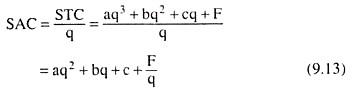
(9.13) gives us that since the STC curve is a third degree curve, the SAC curve would be obtained to be a second degree curve like the curve shown in Fig. 9.7. 

The concave-convex third degree shape of the TVC curve is obtained because of the law of variable proportions (LVP) and this type of shape of the STC curve is obtained because of the shape of the TVC curve, and now the second degree U-shape of the SAC curve is obtained from the shape of the third degree STC curve. It, therefore, follows that the U-shape of the SAC curve is also obtained from the LVP.

The Geometric Method:

We may now see how the U-shape or the second degree shape of the SAC curve can be obtained from the third degree shape of the STC curve with the help of geometry, given in Fig. 9.6.

Along the STC curve of Fig 9.6, the firm’s STC is S₁q₁ at q = qi (or, Oq₁). Therefore, the SAC at q = q₁ would be

SAC = STC/q = S₁q₁/Oq₁ = slope of the guideline OS₁ to the STC curve at q = q₁.

Similarly, at q = q₂, q₃ and q₄, the firm’s SAC would be, respectively, the slopes of the guidelines OS₂, OS₃ and OS₄ (all the guidelines have not been shown in the figure).

Now, it is obvious from Fig. 9.6(a) that as the firm’s q increases, the guideline to its STC curve becomes flatter, i.e., the slope of this line, or the firm’s SAC, decreases. At some q like q = q₅, the guideline, OS₅, would become so flat as to touch the STC curve at the point S₅.

Actually, at q = q₅, the guideline to the STC curve has become the flattest, its slope has been minimum, and so, the SAC is minimum. If q increases beyond q = q₅, the guideline becomes steeper, i.e., its slope increases, and so, the firm’s SAC increases.

From the above analysis, we have obtained that as the firm’s output (q) increases initially, the SAC decreases and at some q (here at q = q₅), the SAC becomes minimum. If q increases beyond this value, the firm’s SAC also increases.

Therefore, the SAC curve of the firm would be U-shaped like the one in Fig. 9.6(b). The SAC curve associated with the STC curve in Fig. 9.6(a) has been shown in Fig. 9.6(b). Here, till q rises to become q = q₅, the SAC curve of the firm has been sloping downward towards right, the SAC curve has reached its minimum at q = q₅, and, as q increases beyond q₅, the SAC curve has been upward sloping towards right.

SAC Curve as the Vertical Summation of the AFC and AVC Curves:

As we know, at any particular quantity (q) of the firm’s output, its short-run total cost (STC) is equal to the sum-total of its total fixed cost (TFC) and total variable cost (TVC), i.e.,

STC = TFC + TVC [eqn. (9.1)]

Now, from (9.1), we obtain

STC/q = TFC/q = TVC/q

or, SAC = AFC + AVC                                            (9.14)

(9.14) gives us that the firm’s SAC curve can be obtained as the vertical summation of its AFC and AVC curves.

The AFC curve of the firm is a rectangular hyperbola (Fig. 9.4) and the AVC curve is a U-shaped curve (Fig. 9.5). We have explained with the help of Fig. 9.8 how we may obtain the SAC curve as the vertical summation of the AFC and AVC curves.

The latter two curves have been given in Fig. 9.8, where we find:

At q = q₁,

SAC = AFC + AVC = F₁q₁ + V₁q₁

= T₁V₁ + V₁q₁ =T₁q₁ (since T₁ has been taken to be a point lying just to the north of V₁ such that T₁V₁ =F₁q₁.)

Therefore, T₁ is a point on the SAC curve. Similarly, at q = q₂, q₃ and q₄, we would obtain, respectively, SAC = T₂q₂, T₃q₃ and T₄q₄, i.e., the points like T₂, T₃ and T₄, would also lie on the firm’s SAC curve. Therefore, the curve joining the points T₁, T₂, T₃ and T₄, would be the firm’s SAC curve. This curve is the vertical summation of the AFC and AVC curves.

In Fig. 9.8, we find that the firm’s SAC curve has been U-shaped. Here from the point of view of geometry also, the cause of this shape is not difficult to understand. Initially, as q increases till q₂, both the AFC and AVC curves slope downwards to­wards right and, therefore, their sum, the SAC curve, also slopes downwards.

At q = q₂, the AVC curve reaches its minimum. Therefore, as q rises beyond q₂, the AVC curve slopes up­ward towards right, but the AFC curve, as a rec­tangular hyperbola, slopes monotonically downward towards right although its rate of fall gradually diminishes.

Now, after q = q₂, as q rises, the rate of rise of the AVC curve would be smaller, for a while, than the rate of fall of the AFC curve resulting in the net a fall in the SAC curve. But now, as q rises, the rate of rise of AVC curve would also rise—reason for this has been given in our explanation of the LVP. But the rate of fall of AFC decreases, since AFC is a rectangular hyperbola.

Therefore, at some q, like q = q₃ in Fig. 9.8, the rate of rise of the AVC curve and the rate of fall of the AFC curve would become equal, and consequently, the rate of fall of SAC would become equal to zero, i.e., the SAC curve would reach its minimum at q = q₃.

As q rises beyond q₃, the rate of rise of AVC would become greater than the rate of fall of AFC resulting in a rise in SAC. Thus, now as q rises beyond q₃, the SAC curve would rise upward towards right. Therefore, we have obtained that as q rises, the SAC curve would be downward sloping to right at first, then it would be upward sloping to right, i.e., the SAC curve would be U- shaped.

The Short-Run Marginal Cost (SMC) and the SMC Curve:

The STC curve is positively sloped, i.e., as the firm’s quantity of output produced (q) rises, its STC also rises. This is because although the fixed cost part of STC remains constant as q rises, the variable cost part of it rises [9.2.7 (i)].

Now, the increment in short-run total cost (STC) of the firm for producing the marginal or the additional unit of a particular quantity of output (q) is known as the short-run marginal cost (SMC) at that q. Similarly, the decrement (negative increment) in STC for reducing the firm’s output (q) by one unit or the marginal unit, is also called the short-run marginal cost (SMC) at that q.) We may write, therefore,

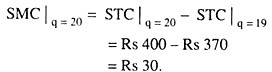
For example, if the STCs at q = 19 units and q Rs 400, then the SMC at q = 20 would be:

Again, by definition, SMC is the rate of change of STC w.r.t. q. So we may write

Again,if q increases by more than one unit, by Δq (Δ1 > 1), then we would have

For if q increases from 20 units to 30 units, and, as a result the STC increases from Rs 400 to Rs 800, then we have

i.e., here SMC is the additional cost for each of the additional 10 units of output.

The short-run marginal cost (SMC) may also be called marginal variable cost (MVC). For, in the short run, increase in STC as a consequence of an increase in q, is actually the increase in TVC, since TFC remains fixed in the short run. For example, as q increases, we obtain from equation (9.1)

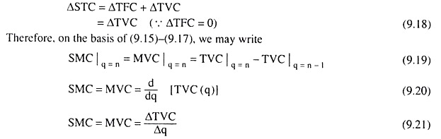
From the SMC function, we obtain what SMC would be at each q. The (q, SMC) combinations that would be obtained from the SMC function may be plotted as points in a (q, SMC) plane. If we join these points by a curve, we would obtain the SMC curve of the firm like the one given in Fig. 9.9.

In the short run, owing to the LVP, the STC curve of the firm would be a third degree curve and, because of this, its SMC curve would be a second degree curve. Let us suppose that the equation of the STC curve is

STC = aq³ + bq² + cq + F [eqn. (9.8]

Here the equation of the associated SMC curve would be

SMC = d/dq (STC) = 3aq² + 2bq + c. (9.21a)

Therefore, if the STC curve is a third degree curve, then the SMC curve would be a second degree or U-shaped curve.

The Geometric Method:

We may explain the point with the help of geometry also. By definition, the firm’s SMC is the slope of its STC curve [eqn. (9.16)]. Again, in the short run, at any q, the slope of the STC curve is equal to that of the TVC curve [9.2.7(ii)].

Therefore, the slope of the TVC curve at any q may also be taken to be the SMC. Now, in Fig. 9.3, we see that owing to the LVP, both the STC and TVC curves are concave downwards at first, then they are convex downwards.

That is, as q increases initially, the slopes of both the STC and TVC curves would diminish, i.e., the SMC would diminish, and then the slopes of both the curves would increase, i.e., SMC would increase. Therefore, the SMC curve also would be U-shaped because of the LVP.

In Fig. 9.3(b), at q = q₀, or at the points H₀ and G₀, the concave portions, respectively, of the STC and TVC curves have reached their ends, i.e., at these two points the slopes of these two curves have been minimum, i.e., the SMC has become the minimum.

The SMC curve associated with the STC and TVC curves of Fig. 9.3(b) have been given in Fig. 9.3(c). It may be noted here, and that the minimum point of the SMC curve corresponds to the maximum point of the marginal product (MP) curve of the variable input(s).

Similarly, it can be seen in Fig. 9.3 that, as q increases from 0 to q₀, the MP of variable inputs (slope of TP_V curve) is rising and the MC (slope of TVC) is falling, and, as q rises from q₀ to q₁, the MP_V is falling and the MC is rising, i.e., the rising segment of the MP_V curve (shaped like the MP_L curve in Fig. 8.2, not shown in Fig. 9.3) corresponds to the falling segment of the MC_L curve; and the falling segment of the MP_V curve corresponds to the rising segment of the MC curve.

Relation between SMC, SAC and AVC:

Relation between SMC and SAC:

We may first explain the relation between marginal cost and average cost with the help of a simple example. Let us suppose, when the firm produces 9 units of its product, its total cost (STC) is Rs 54. Here we get the average cost (SAC) at q = 9 to be equal to 54/9 = 6 (Rs). Now, if the firm produces 10 units of output, then the resulting increase in its total cost would be its marginal cost (SMC) at q = 10 units.

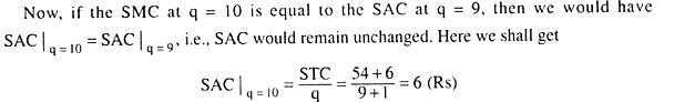
That is, what we have obtained here is that if SMC = SAC, when q increases, then the SAC would remain unchanged.

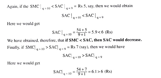
That is, if SMC > SAC, then SAC would increase.

On the basis of the above examples, we obtain the following relations between the average cost and marginal cost:

(i) If, as q increases, SMC remains the same as SAC, then SAC would remain unchanged. Conversely, if SAC remains unchanged as q increases then SMC would be equal to SAC.

(ii) If, as q increases, SMC is obtained to be less than SAC, then SAC would fall. Con­versely, if SAC falls as q increases, then SMC must have been smaller than SAC.

(iii) If, as q increases, SMC becomes greater than SAC, then SAC would rise. Conversely, if SAC increases as q rises, then SMC must have been greater than SAC.

We have constructed the SMC and SAC curves in Fig. 9.10 on the basis of the above relations. In this Figure, the point N is the minimum point of the U-shaped SAC curve with q = q₁. At the minimum point N, if q increases by a very (infinitesimally) small amount, SAC remains unchanged.

Therefore, from SAC-SMC relation (i), we obtain that at the minimum point N (q = q₁) on the SAC curve, SAC would be equal to SMC. That is, the point N itself would be the point of intersection between the SAC and SMC curves.

Second, in Fig. 9.10, at any point on the SAC curve to the left of its minimum point, N, i.e., for q < q₁ SAC decreases as q increases. Therefore, from the SAC-SMC relation (ii), we obtain that, for q < q₁ or to the left of the minimum point N, SMC would be less than SAC (SMC < SAC), i.e., the SMC curve would lie below the SAC curve.

Finally, at any point on the SAC curve to the right of its minimum point N, i.e., for q > q₁, SAC increases as q increases. Therefore, from the SAC – SMC relation (iii), it follows that for q > q₁, or, to the right of the minimum point N, SMC would be greater than SAC (SMC > SAC), i.e., SMC curve would lie above the SAC curve.

In the above analysis, owing to the SAC – SMC relations, first, the SMC curve would lie below the SAC curve to the left of the minimum point of the latter curve which is U-shaped. Second, the SMC curve would intersect the SAC curve at the latter’s minimum point.

Lastly, the SMC curve would be above the SAC curve to the right of the latter’s mini­mum point. In other words, the SMC curve would intersect from below the SAC curve at the latter’s minimum point N and then it would go above the latter curve (i.e., the SAC curve).

That is, the SMC curve is upward sloping at the point N and, since this curve is U-shaped, it must have reached its minimum somewhere to the southwest of the point N. In Fig. 9.10, the mini­mum point of the SMC curve is point H where the firm’s q is q = q₃ (q₃ < q₁).

The relation that we have obtained above between SMC and SAC is known, in general, as the marginal-average relation. This relation is applicable to short-run cost as it is applicable to long-run marginal and average cost.

Similarly, it is applicable marginal variable cost and aver­age variable cost, marginal revenue and average revenue, marginal product and average prod­uct, marginal revenue product and average revenue product, and so on.

The main points of this relation are:

(i) If M (marginal) < A (average), then A would fall. So when A falls we have, M < A.

(ii) If M > A, then A would rise. So when A rises, we have, M > A.

(iii) If M = A, then A would remain unchanged. So, if A remains unchanged, we have, M = A.

Relations between SMC and AVC:

The short-run marginal cost (SMC) and the marginal variable cost (MVC) are the same—at any particular q, MVC itself is the SMC. Therefore, the relation between SMC and AVC is actually the relation between MVC and AVC, and the usual marginal-average relation applies here.

Since both the SMC (or MVC) and the AVC curves are U-shaped, the relation between these curves would be obtained if we replace SAC and SMC by AVC and MVC (= SMC), respectively.

The points of relation be­tween SMC (= MVC) and AVC would be the same as the three points of relation between SMC and SAC. Also, the points of relation between the SMC (= MVC) and AVC curves would be the same as those between the SMC and SAC curves.

The relation between the SMC (= MVC) and AVC curves may be mentioned here with reference to Fig. 9.10. Here G is the minimum point of the U-shaped AVC curve with q = q₂. At G, the SMC curve would intersect the AVC curve. To the left of the point G, the SMC curve would lie below the AVC curve and to the right of G, the SMC curve would lie above the AVC curve.

The SMC curve would intersect the AVC curve at point G from below and then would go above the AVC curve upwards towards right, which means the U-shaped SMC curve is upward sloping at point G and must have reached its minimum at some point to the southwest of G. In Fig. 9.10, this point is the point H, where the output of the firm is q₃ (q₃ < q₂).

Relative Positions of the Minimum Points of the SAC, AVC and the SMC curves:

We have obtained that owing to the law of variable proportions (LVP), the SAC, AVC and SMC curves are all U-shaped. The upward sloping portion of the SMC curve would intersect both AVC and SAC curves at their minimum points (Fig. 9.10). It may also be noted that the AVC curve throughout its length lies below the SAC curve.

This is because at any q we have:

STC = TFC + TVC

⇒ STC > TVC (.^.. TFC > 0)

⇒ STC/q > TVC/q

⇒SAC > AVC, or, AVC < SAC

Now, since the AVC curve lies below the SAC curve, the upward sloping portion of the SMC curve first intersects the AVC curve and then intersects the SAC curve at their respective minimum points G and N.

From this we obtain that the minimum point of the SMC curve, H, lies to the southwest of the minimum point G of the AVC curve, and the latter point, i.e., G, lies to the southwest of the minimum point N of the SAC curve.

We shall, therefore, obtain:

q₃ < q₂ < q₁

or q₁ > q₂ > q₃

where q₁, q₂ and q₃ are, respectively, the outputs at the minimum points N, G and H of the SAC, AVC and SMC curves.

Relations between SMC, SAC and AVC—Mathematical Derivation:

Relation between SMC and SAC:

Now, as we know, the firm’s SAC, AVC and SMC, all three curves are U-shaped because of the law of variable proportions (LVP). In Fig. 9.10, the minimum points of these curves are, respectively, N, G and H, and the quantity of output at these three points are, respectively, q₁, q₂ and q₃.

Now we may determine the relation between the SMC and SAC curves with the help of Fig. 9.10.

Since the SAC curve is U-shaped and the output at the minimum point, N, of this curve is q₁ we obtain

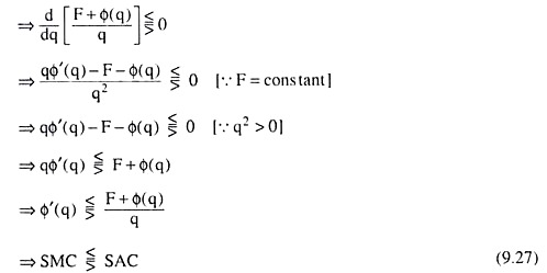
(9.27) gives us:

(i) At the minimum point N, of the SAC curve, when q = q₁, we would have SMC = SAC, i.e., the SMC curve would intersect the SAC curve at the latter’s minimum point, N.

(ii) To the left of the minimum point N of the SAC curve, when q < q₁, we would have SMC < SAC, i.e., the SMC curve would lie below the SAC curve.

(iii) Lastly, to the right of the minimum point N of the SAC curve when q > q₁ we would have SMC > SAC, i.e., the SMC curve would lie above the SAC curve.

(iv) From (i), (ii) and (iii) above, it is obvious that, at the minimum point N of the SAC curve, the SMC curve would be sloping upward towards right. Therefore, the minimum point H of the U-shaped SMC curve must lie somewhere to the southwest of the point N. That is why, at the point H, we obtain q = q₃ < q₁.

Relation between SMC and AVC:

In Fig. 9.10, at the minimum point G of the U-shaped AVC curve, the output of the firm is q = q₂. At this point, we obtain

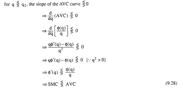
Eqn. (9.28) gives us:

(i) At the minimum point G of the AVC curve, when q = q₂, we would have SMC = AVC, i.e., the SMC curve would intersect the AVC curve at the latter’s minimum point G.

(ii) To the left of the point G, when q < q₂, we would get SMC < AVC, i.e., the SMC curve would lie below the AVC curve.

(iii) To the right of the point G, when q > q₂, we would obtain SMC > AVC, i.e., SMC curve would lie above the AVC curve.

(iv) From (i)-(iii) above, it is obvious that at the minimum point G of the AVC curve, the SMC curve would be upward sloping, Therefore, the minimum point H of the U-shaped SMC curve must lie somewhere to the southwest of the point G. Therefore, at the point H, we would have q = q₃ < q₂.

Relative positions of the minimum points of the SAC, AVC and SMC curves:

In Fig. 9.10, the minimum points of the SAC, AVC and the SMC curves are, respectively, N (q = q₃), G (q = q₂) and H (q = q₃). Before determining the relative positions of these three points, let us remember that by definition, AVC < SAC at any q, and so the entire AVC curve would lie below the SAC curve [9.2.13(c)].

Now, as we know owing to LVP the SMC curve is U-shaped. That is why in Fig. 9.10, the SMC curve is upward sloping after its minimum point H. Again, from the SMC-SAC relation (iv) and the SMC-AVC relation (iv), we obtain that the minimum points G and N of the AVC and the SAC curves lie on the upward sloping portion of the SMC curve.

Now, since the entire AVC curve lies below the SAC curve, the SMC curve—while going upwards—-would first intersect the AVC curve at the latter’s minimum point G and then intersect the SAC curve at this curve’s minimum point N.

We, therefore, obtain that the minimum point G of the AVC curve would lie to the southwest of the minimum point N of the SAC curve, and the minimum point H of the SMC curve would lie to the southwest of the minimum point G of the AVC curve.

That is, we obtain

q₂ < q₁ and q₃ < q₂

=> q₃ < q₂ < q₁                                   (9.29)