Long Run Cost of a Firm | Microeconomics

In this article we will discuss about the long run cost of a firm, explained with the help of suitable diagrams. 

In the short run, the firm may change its quantity of output produced (q) by means of suitable changes in the quantities used of different variable factors, but it cannot change the quantities used of the fixed factors. The cost of producing the firm’s output under the circumstances of the short run, is called the short-run cost of production.

On the other hand, if the firm produces a particular quantity of output after making required changes in both the variable and fixed factor inputs under the circumstances of the long run, then the cost of producing the output is called the long-run cost of production.

For example, if the firm increases its output in the short run from 400 units to 500 units per day and if the cost of producing this 500 of output is Rs 5,000, then this cost is the short-run cost of production. Here, in order to increase q, the firm has suitably changed the use of the variable inputs, but it has not been possible for it to make the required changes in the fixed inputs.

If the firm was allowed a long run of time to change the fixed input quantities suitably, then this cost would have been, say, Rs 4,500, and, in that case, this cost would have been called the long-run cost of production.

We are assuming here, of course, that the prices of all the inputs remain unchanged. In the long run also, like the short run, cost of production may be expressed as total cost, average cost and marginal cost.

From Short-Run Total Cost (STC) to Long-Run Total Cost (LTC)—Relation between STC and LTC Curves:

In the short run, the total cost of producing a particular quantity output can be known from the STC curve. Similarly, in the long run, the total cost of any output can be known from the LTC curve. We shall now see that the firm’s LTC curve can be derived from its STC curves. We may explain this with the help of Fig. 9.11.

Different STC Curves for Different Amounts of Total Fixed Cost (TFC):

In Fig. 9.11, we see that, if, in the short run, the TFC of the firm is F₁ (or OF₁), then its STC curve is STC₁. However, if the firm had more of fixed inputs in the short run, its TFC would have been greater, say, F₂ (> Fi), and it STC curve would have been different, say, STC₂.

Similarly, if the firm’s TFC were F₃ or F₄ (F₄ > F₃ > F₂ > F₁) its STC would have been, respectively, STC₃ or STC₄. We may say, therefore, that the firm’s STC curve would be different for a different amount of TFC. In Fig. 9.11, we have shown only four STC curves of the firm corresponding to four different amounts of TFC.

We have to remember, however, that, actually, the firm would have only one of these different amounts of TFC in the short run, and it would have only one STC that is obtained at that TFC. That is, in the short run, it is not possible for the firm to have more than one STC curve or to move from one STC curve to another.

For that would mean changing the TFC or changing the quantities of the fixed inputs, which is not possible in the short run.

Relative Positions of the STC Curves:

It is important to remember certain points regarding the relative positions of the STC curves. For example, let us speak of the first two STC curves of Fig. 9.11. The fixed input quantities for the STC₂ curve are larger than those for the STC] curve. For these two curves we obtain

STC₁ = TFC₁ (= F₁ = Constant) + TVC₁

STC₂ = TFC₂ (= F₂ = Constant) + TVC₂

Here STC₁ = amount of STC at any q along the STC₁ curve

TFC₁ = amount of TFC in STC₁

TVC₁ = amount of TVC in STC₁

Also, STC₂ = amount of STC at any q along the STC₂ curve

TFC₂ = amount of TFC in STC₂

TVC₂ = amount of TVC in STC₂

From above, we obtain STC₂ – STC₁ = (F₂ – F₁) – (TVC₁ – TVC₂) (9.30)

In Fig. 9.11, we find that, at any q, TFC is smaller in STC| than STC₂ by the amount, F₂-F₁ = constant. At a very small q, the TVC would almost be the same for the two STC curves, and so STC) would be less than STC₂ by the amount which is almost equal to F₂ – F₁, and the STC, curve would lie below the STC₂ curve.

But as q rises, both TVC) and TVC₂ would rise (at a decreasing rate, because of LVP), but the rate of increase of TVC₂ would be smaller than that of TVC₁. For, the fixed input quantities with the STC₂ curve are larger, and so, in the case of this curve, the variable inputs can be used more efficiently by applying division and specialisation of labour.

As a consequence, as q rises, we would have TVC₁ >TVC₂, (TVC₁ -TVC₂) increasing and, therefore, (STC₂ – STC₁) decreasing [by virtue of eqn. (9.30)] (initially, STC₂ – STC, = almost F₂ – F₁).

That is, as q rises, the vertical gap between the STC₂ and STC₁ curves would be decreasing, till at some q, e.g., at q = q₁ in Fig. 9.11, this gap would become zero, i.e., we would have, STC₁ = STC₂, i.e., STC, and STC₂ curves would intersect each other. In other words, at q = q₁, the amount by which F₂ exceeds F, would exactly be equal to the amount by which TVC, would exceed TVC₂, i.e., at q = q₁, we would get, F₂ – F₁ = TVC₁ – TVC₂.

Now, as q increases beyond q₁, the shortage of fixed inputs in the case of the STC₁ curve would be felt more than in the case of the STC₂ curve. Therefore, the rate of increase in TVC₁ would be larger than that in TVC₂, as q increases.

Therefore, now (TVC₁ -TVC₂) would be larger than (TFC₂-TFC₁) which is a constant = F₂-F₁. As a result, now we would have STC₁ > STC₂, and so the STC₁ curve would lie above the STC₂ curve.

Therefore, in the above analysis, in the case of a relatively small output, e.g., in Fig. 9.11, for q < q₁, the STC₁ curve would lie below the STC₂ curve, and in the case of a relatively large output, e.g., for q > q₁, the STC, curve would go above the STC₂ curve, after intersecting the latter.

The two curves would intersect at q = q₁. The simple explanation that we have given here of the relative positions of different STC curves with different TFCs, would apply to any two STC curves, one with a smaller TFC and the other with a higher TFC.

From Short-Run Total Cost to Long-Run Total Cost:

Now if the STC curve of the firm be STC, and if it produces at present, i.e., in the short run, an output of Oc in Fig. 9.11, then its STC would be b,c. But if the firm’s STC curve were STC₂, then its STC at q = Oc would have been b₂c (b₂c < b₁c). In fact, of the four STC curves given here, if the firm had the STC₂ as its STC curve, then the cost of producing Oc of q in the short run, would have been the lowest, viz., b₂c.

Therefore, if the firm continues to produce Oc per period, then, in the long run, the firm would increase its fixed input quantities appropriately so that its TFC would increase from F₁ to F₂, and it could shift from the STC, curve to the STC₂ curve.

In general, it may be said that if the firm goes on producing Oc of output and if its STC curve be one other than STC₂, then in the long run, the firm by suitably changing its fixed input quantities, may shift from its present STC curve to the STC₂ curve. Therefore, the cost of producing the output of Oc in the long-run, i.e., the long-run cost (LTC), would be b₂c.

The LTC Path of the Firm:

It is obvious from the discussion above that if the output of the firm (q) is between 0 and q₁ in Fig. 9.11 (i.e., at 0 < q < q₁) then in the long run the firm would want to remain on the F₁T₁ segment of the STC, curve. Similarly, at q₁ < q < q₂ and at q₂ < q < q₃, the firm would want to remain on the T₁T₂ segment of the STC₂ curve and on the T₂T₃ segment of the STC₃ curve, respectively.

Lastly, if q > q₃, the firm would want to remain on the segment of the STC₄ curve that lies to the right of the point T₃. Therefore, the firm would be able to know the cost of production at any output in the long run from the path which would be obtained by joining the segments F₁T₁, T₁T₂, T₂T₃, T₃T₄, etc. of the different STC curves.

Therefore, we may call this path the long run total cost (LTC) path. This path is not a continuous curve, as is evident in Fig. 9.11. Since, here we have only four STC curves, the LTC path obtained would consist of four different scallops, viz., F₁T₁, T₁T₂, T₂T₃ and T₃T₄ and there are three kinks on this path at points T₁, T₂ and T₃.

The LTC Curve of the Firm:

But, if we assume theoretically that the total fixed cost (TFC) of the firm is a continuous variable, then we would obtain an indefinitely large number of STC curves corresponding to an equal number of values of TFC. In that case, each scallop of the LTC path would be ultimately reduced to a point and the LTC path, in the limit, would be reduced to the LTC curve of the firm. We have shown the LTC curve thus obtained in Fig. 9.12.

The LTC curve that has been obtained here is made up of the points of an indefinitely large number of STC curves, each such curve contributing a point to the LTC curve. In mathematics, this type of curve is known as an envelope curve. Here each contributing STC curve touches the LTC curve at one point only.

LTC ≤ STC

We may easily understand from Fig. 9.12 that at any particular output, q = q*, of the firm we would obtain LTC ≤ STC. Here each of the STC₁, STC₂, STC₃. . . curves may be the STC curve of the firm. However, in the short run, only one of these curves would be the firm’s STC curve, depending on the quantities of the fixed inputs, i.e., on TFC.

Let us suppose that the firm intends to produce a particular quantity, q*, of its output. It is obvious in Fig. 9.12 that the long-run total cost (LTC) of producing q* of output is dq*. Again, the short-run total cost (STC) at q = q* may also be dq*, if the firm’s STC curve is STC₃.

That is, if the firm’s STC curve is STC₃, then at q = q*, we would obtain LTC = STC. But if the firm’s STC curve is any-one other than STC₃, if it is STC₁ or STC₂ or STC₄, etc., then it is evident from Fig. 9.12 that the short-run cost of production at q = q* would be greater than the long-run cost, dq*. Therefore, we have obtained that, at any q, LTC ≤ STC.

From Short-Run Average Cost (SAC) to Long-Run Average Cost (LAC):

Relation between SAC Curve and LAC Curve:

The short-run average cost (SAC) of the firm at any q, as we know, is the SAC per unit of output, and it is obtained as SAC = STC/q. Similarly, the long-run average cost (LAC) of the firm at any q is the LAC per unit of output, and it is obtained as LAC = LTC/q.

Also, the firm’s short-run average cost (SAC) at any q can be obtained from its SAC curve. Similarly, its long-run average cost (LAC) at any q may be obtained from its LAC curve. We shall now see how this LAC curve of the firm can be obtained. We shall see that the LAC curve can be obtained from the firm’s SAC curves just as, the LTC curve can be obtained from the firm’s STC curves.

Different SAC Curves for Different Amounts of TFC:

For different sets of fixed input quantities, i.e., for different plant sizes with different TFCs, we obtain different third degree STC curves. We also know that each STC curve has its associated U-shaped SAC curve.

We may say, therefore, that we shall obtain different SAC curves for different plant sizes i.e., for different amounts of TFC. In Fig. 9.13 We have shown five SACs for five different plant sizes. The relative position of these curves would be like those given in Fig. 9.13. As the plant size, or, TFC increases, the SAC curve would shift to the right from SAC₁ to SAC₂, from SAC₂ to SAC₃, from SAC₃ to SAC₄, and so on.

Relative Position of the SAC Curves:

The relative positions of the SAC curves may be derived from the relative positions of the STC curves. For example, in Fig. 9.13, let us consider the curves SAC₁ and SAC₂.

If the fixed input quantities and the TFC are larger for SAC₂ than for SAC₁, then the relative position of these two curves would be like that shown in Fig. 9.13, i.e., for relatively smaller output quantities, the SAC₁ curve would lie below the SAC₂ curve and for relatively larger quantities of output, the SAC, curve would go above the SAC₂ curve. We may explain this in the following way.

Let us assume that the STC curves associated with the SAC₁ and SAC₂ curves of Fig. 9.13(b) are, respectively, the STC₁ and STC₂ curves of Fig. 9.13(a). Here the STC₁ and STC₂ curves have intersected at q = q₁, and so at the same q₁ the SAC, and SAC₂ curves would also intersect.

For, at q = q₁:

STC₁ = STC₂

=> STC₁/q₁ = STC₂/q₁

=> SAC₁ = SAC₂

Now, while discussing the relative positions of the STC curves, at any q, we shall obtain

STC₂ – STC₁ = TFC₂ – TFC₁ + TVC₂ – TVC₁ [eqn. (9.30)]

We have said that at a very small q, TVC₁ and TVC₂ are almost equal, and so we may write

STC₂ – STC₁ = TFC₂ – TFC₁ (= constant)

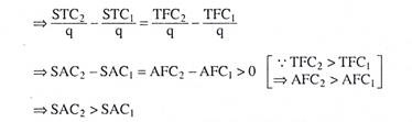
We have obtained, therefore, that when q is very small, the SAC, curve would lie below the SAC₂ curve and the vertical gap between these two curves at that q would be almost the same as the difference between AFC₂ and AFC₁.

Now, in the discussions, as q increases, TVC₁ and TVC₂, both would increase, TVC₂ remaining smaller than TVC₁, and (TVC₁ -TVC₂) would gradually increase. All this is because of division and specialisation of labour. Eventually, at some q (e.g., q = q₁ in Fig. 9.11) we would get

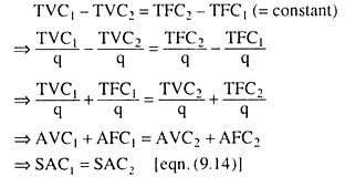
That is, at some q (= q₁ in Fig. 9.11), SAC₂ would become equal to SAC, because of economies of scale, i.e., SAC, and SAC₂ curves would intersect each other. If q increases beyond that, i.e., at q > q₁ (in Fig. 9.11), we would get

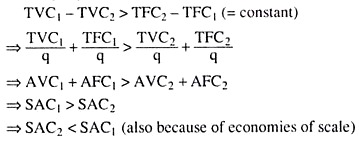
That is, in Fig. 9.13, if q > q₁, the SAC₁ curve would lie above the SAC₂ curve. The explanation that we have given here of the relative position of the SAC₁ and SAC₂ curves would also apply to the relative position of SAC₂ and SAC₃ curves, of SAC₃ and SAC₄ curves, and so on.

Another point about the relative position of the SAC curves is that, as the firm moves on from a lower TFC to a higher TFC, i.e., as it moves on from a smaller plant size to a larger plant size, the SAC curve goes on shifting downward towards right up to a certain point and then would be shifting upward towards right.

For example, in Fig. 9.13(b), first the SAC curve has shifted downward towards right from SAC₁ to SAC₂ to SAC₃ and then it has shifted upward towards right from SAC₃ to SAC₄ to SAC₅.

The reason for this is that, initially, as the size of the plant increases, the firm’s SAC diminishes up to larger quantities of output and towards a lower minimum, owing to the economies of scale, and so, the minimum point of a particular SAC would be positioned downward towards right of the minimum point of the SAC to the left of it. In Fig. 9.13, this has occurred up to the SAC₃ curve.

That is why we obtain: q₃‘ > q₂‘ > q₁‘ and L₃q’₃ < L₂q’₂ < L₁q’_1. If the size of the firm’s plant increases beyond SAC₃, we would obtain that SAC with a larger plant diminishes up to a larger quantity of output because of economies of scale but towards a higher minimum because of the diseconomies of scale (9.3.4, 9.3.5). That is why we obtain q’₅ > q’₄ > q’₃ and L₅q’₅ > L₄q’₄ > L₃q’₃.

From SAC to LAC:

In Fig. 9.13, if the firm’s SAC curve is SAC₁ and if it produces at present (i.e., in the short run), an output of q* per period, then its SAC would be a₁q*.

But if the firm’s SAC curve were SAC₃, then the SAC of producing the output of q* would have been a₃q* (< a₁q*). In fact, of the five SAC curves given in Fig. 9.13, the cost of producing q* of output is minimum (= a₃q*) on the SAC₃ curve. Therefore, if the firm goes on producing q* of output then in the long run, it would shift from the SAC₁ to the SAC₃ curve.

Generally speaking, if the firm produces an output of q* per period and if its SAC be a curve other than SAC₃, then in the long run, it would shift to the SAC₃ curve after making suitable changes in the fixed input quantities. Therefore, the long-run average cost (LAC) of q = q* would be a₃q*.

The LAC Path of the Firm:

It is evident from the above discussion that if, in Fig. 9.13, the quantity of output is between 0 and q₁ (0 < q < q₁), then in the long run, the firm would remain at some point on the portion of the SAC, curve to the left of the point K₁.

Again, for q₁ < q < q₂, the firm would remain at some point on the K₁K₂ portion of the SAC₂ curve. Again, for q₂ < q < q₃, and for q₃ < q < q₄, the firm would want to remain, respectively, on the K₂K₃ portion of the SAC₃ curve and on the K₃K₄ portion of SAC₄ curve. Lastly, for q > q₄, the firm would remain at some point on the SAC₅ curve to the right of the point K₄.

On the basis of the above discussion, we may say that the LAC at any particular q can be obtained from the AK₁ K₂ K₃ K₄B path. Therefore, this path may be called the LAC path of the firm. Like the LTC path of Fig. 9.12, this path also is not a continuous curve.

Since we have shown here only five SAC curves, this path is made up of five scallops, viz., AK₁, K,K₂, K₂K₃, K₃K₄ and K₄B, and there are four kinks on this path at the points K₁, K₂, K₃ and K₄.

The LAC Curve of the Firm:

Theoretically, if we assume that the TFC of the firm can vary continuously (in the long run), then for the indefinitely large number of values of TFC, we shall obtain an indefinitely large number of SAC curves. In that case, each scallop on the LAC path would be ultimately reduced to a point, and the LAC path, in the limit, would be reduced to the LAC curve of the firm.

We have shown the LAC curve thus obtained in Fig. 9.14. The LAC curve obtained here is made up of the points of an indefinitely large number of SAC curves, each such curve contributing a point to the LAC curve. Like the envelope LTC curve, the LAC curve also is an envelope curve—it is an envelope of the SACs. Here the LAC curve touches each contributing SAC curve at only one point.

LAC ≤ SAC:

We may now easily see, with the help of Fig. 9.14, that any particular output quantity q = q*, the firm would have LAC ≤ SAC, i.e., the long-run average cost at any q is either less than or equal to the short-run average cost. Now, each of the SAC curves given in Fig. 9.14 may be the firm’s SAC curve.

However, in the short run, only one of these curves can be the firm’s SAC curve, depending on the quantities of the fixed inputs currently possessed by the firm, i.e., on the TFC that the firm has to bear at present. Let us suppose that the firm intends to produce a particular quantity of output, q*, of its output. It is obvious in Fig. 9.14 that the LAC of this q is a₃q*.

Again, at q = q*, the SAC also may be equal to a₃q* if the firm’s SAC curve is SAC₃. That is, if the firm’s SAC curve is SAC₃, then at q = q*, the firm would have LAC = SAC. But if the SAC curve of the firm is any of the SAC curves other than SAC₃, then SAC of producing q* of output would be greater than a₃q* (= LAC).

That is at q = q*, the firm’s SAC would be equal to LAC (if the SAC curve is SAC₃) or SAC would be greater than LAC (if the SAC curve is any-one other than SAC₃). That is, we have obtained, at any q (= q* here), LAC ≤ SAC.

Explanation of the Shapes of the Long-Run Total Cost (LTC) Curve and the Long- Run Average Cost (LAC) Curve:

As we have obtained in Fig. 9.12, the firm’s LTC curve, like its STC curves, is a third degree curve—concave downwards initially, then convex downwards. However, the reasons for the same kind of shape of the STC and LTC curves are not the same.

As we know, the concave- convex shape of the STC curve is obtained from the law of variable proportions (LVP). On the other hand, the concave-convex shape of the LTC curve is obtained owing to economies and diseconomies of scale.

We have to remember here that although both the STC and LTC curves are of the same type of shape, STC > 0 and STC = TFC at q = 0, but LTC = 0 at q = 0. The reasons are obvious. In the short run, even if nothing is produced (q = 0), fixed costs cannot be avoided.

On the other hand, in the long run, all the factors are variable. So when nothing is produced (q = 0), employment of all the factors is reduced to zero, and so LTC is reduced to zero. If the total cost curve is of third degree, i.e., at first concave downwards and then convex downwards, then the average cost curve would be a U-shaped or a second degree curve.

Therefore, if the LTC curve is concave-convex owing to the economies and diseconomies of scale, then the LAC curve associated with the LTC curve would also be U-shaped. We have shown a LTC curve and its associated LAC curve in Fig. 9.15. At q = q₀, the guideline OG, to the LTC curve, has been a tangent to the curve [Fig. 9.15(a)]; that is why, at q = q₀, the LAC would be minimum [Fig. 9.15(b)].

Economies and Diseconomies of Scale:

As the firm’s plant size and TFC and its scale of operation increases in the long run, certain economies of scale are usually obtained. In other words, since in the long run the firm can adjust all inputs optimally, it can reduce the unit cost of production by changing its plant-size.

Adam Smith (1723-90) gave one of the outstanding reasons for this, which is known as division and specialisation of labour. According to Smith, when the number of workers increases in the short run, fixed inputs remaining fixed, the opportunities for specialisation and division of labour are rapidly exhausted.

The firm certainly moves along the convex downward portion of its total product curve [Fig. 8.2(a)], i.e., marginal product of labour certainly rises, but not for long. The marginal product curve of labour quickly reaches its maximum, and then declines [Fig. 8.2(b)].

But in the long run, when workers and fixed inputs increase together, division of labour can be expanded indefinitely and the workers may get specialised in different jobs. As a result, the firm’s unit cost of production reduces indefinitely owing to division and specialisation of labour.

Then there are some technological reasons for obtaining the economies of scale in the long run. It has been observed, for example, that a machine with ten times more of production capacity does not require ten times more of money as its price, nor does it require ten times more of building space, ten times more of labour to work with, and so on.

This means, in the long run, if the firm increases the size of its equipment, its average cost of production will diminish. Technological economies may be obtained in other forms also.

For example, let us suppose that the firm uses two types of machines—one is used for producing its output and the other for packaging its product. The first machine produces, say, 12,000 units of output per day and the second machine packages, say, 10,000 of the product per day.

Now, if the firm’s output is 24,000 units per day, it would require two units of the first machine and three units of the second machine, and would have 6,000 units of packaging capacity unutilized.

This is, of course, a short run problem. In the long run, the firm may increase the quantity of the first machine to five and that of the second machine to six, and its output quantity to 60,000 units. Thus, the firm would be able to combine the two types of machine in such a way that there would be no excess capacity. As a result, the firm’s unit cost would reduce in the long run.

Therefore, that the division and specialisation of labour and technological factors are two broad forces that would enable the firm to enjoy economies of scale in the long run, i.e., to reduce the unit cost of production by increasing its scale of operation. These forces give rise to the negatively sloped or downward sloping portion of the firm’s LAC curve [Fig. 9.15(b)].

Let us now come to diseconomies of scale which arises actually from limitations to efficient management. The essentials of managing any business consist of controlling and coordinating a wide variety of activities like production, transportation, finance, sales, and so on. To perform the managerial function of coordination and control, the manager must have accurate information. He must not take decisions in ignorance.

Now, in the long run, as the scale of the plant expands beyond a certain capacity, top management necessarily has to delegate responsibility and authority to lower category employees. As a result, direct contact and control tend to be lost and efficiency of operation tends to decline.

Red tape and paper work now expand—they now take the place of direct decision-making. Management is generally not as efficient. The cost of performing the managerial function increases, and also the unit cost of production.

It is very difficult to determine when diseconomies of scale set in and when they become strong enough to outweigh the economies of scale and to push the firm along the upward sloping portion of its LAC curve. There are some businesses where economies of scale are negligible, and diseconomies may soon come to dominate as the plant-size increases in the long run. Fig. 9.16(a) shows an LAC curve for a firm of this type.

Fig. 9.16 Relative importance of economies and diseconomies of scale Again, there are some other businesses where the economies of scale are extremely important. Even after the efficiency of management begins to decline, technological and other economies of scale may overpower the diseconomies over a wide range of output.

Thus, in such a case, the LAC curve may not become upward sloping until a very large volume of output has been attained. This case is typical of the so-called natural monopolies. The LAC curve here would be like the curve shown in Fig. 9.16(b).

In many actual situations, however, neither of these two extremes dominates. In this case, until the volume of output is very great the economies may be able to offset the diseconomies. So the LAC curve here would have a long horizontal segment as shown in Fig. 9.16(c).

Correspondence between the Points on the Firm’s Long-Run Expansion Path and the Points of Tangency of the Envelope LTC and LAC Curves with the STC and SAC Curves:

Let us suppose that a firm uses only two inputs, X₁ and X₂, to produce a single output. In the long run both the inputs are variable. The long-run production function of the firm is

q = f(x₁, x₂).

In Fig. 9.18, the firm’s isoquant (IQ) map and the iso-cost lines (ICLs) are given. The prices of the inputs remaining constant, the firm’s iso-cost lines are parallel to each other. In this figure the long-run expansion path (LEP) of the firm is shown to be OE. It starts from the origin and passes through the points of tangency between the isoquants and the iso-cost lines.

The points on the expansion path give us minimum amounts of cost at the given levels of output. For example, it gives us that q₁, q₂ and q₃ of output can be produced at the minimum costs of C₁, C₂ and C₃, respectively.

These (C, q) combinations are given implicitly at the points F₁, F₂ and F₃, respectively. If we now explicitly plot these (C, q) combinations as the points G₁, G₂ and G₃ in a separate diagram, say, Fig. 9.19, then the curve passing through these points would be the long-run (total) cost (LTC) curve of the firm.

Therefore, that there is a one-to-one correspondence between the points on the long-run expansion path (LEP) of the firm and its long-run total cost (LTC) curve. We have obtained here the points G₁, G₂, G₃, etc. on the LTC curve corresponding, respectively, to the points F₁, F₂, F₃, etc. on the firm’s LEP.

Also, as we know, the long-run average cost (LAC) at any particular quantity of output is obtained by dividing the LTC by that quantity. In other words, there is also a one-to-one correspondence between the points on the LTC and the LAC curves. Therefore, we may say that there is a one-to-one correspondence between the points on the LEP, LTC and LAC curves.

Also, since the points on the envelope LTC and LAC curves are respectively the points of tangency with the STC and SAC curves, we may say then that there is one-to-one correspondence between the points on the LEP and the points of tangency of the LTC curve with the STC curves and those of the LAC curve with the SAC curves.

Therefore, the envelope curve approach of obtaining the LTC and LAC curves and the expansion path approach of the obtaining the LTC and the LAC curves are really one and the same.

We may now see with the help of Fig. 9.18, why and when the firm may not remain on its LEP and what the consequences would be. If the firm wants to produce q₂ of output at the minimum possible cost—which is here C₂, then the firm would have to remain at the point F₂ on its LEP, for F₂ is the point of tangency between the IQ₂ and the ICL₂ curves.

At the point F₂, the firm uses x” of input X₁ and x”₂ of input X₂. Now if the quantity of X₂ is fixed at x₂ in the short run and X₁ is a variable input, the firm would have no difficulty to remain at the point F₂ on its LEP, for here it has the required quantity x₂ of X₂.

At the point F₂, we obtain the firm’s STC and LTC to be equal, both being equal to C₂. But with a fixed quantity of x₂ of input X₂ and with the required quantity of X₁, viz., AH₃, if the firm wants to produce the output q₃ in the short run, then it would have to remain at the point H₃ using AH₃ of X_P But the point H₃ is not on the firm’s LEP.

The STC in this case of producing q₃ of output would be given by the iso-cost line that passes through the point H₃ (not shown in Fig. 9.18). But in the long run, when both the inputs are variable, the firm would use x₂” of X₂ and x”‘₁ of X₁ to produce q₃ of output at the point F₃ on IQ₃.

In this case, the firm would be able to produce q₃ of output at the minimum possible cost, C₃, given by the iso-cost line ICL₃, since this line is a tangent to IQ₃ at the point F₃. Also, since the ICL passing through H₃ is higher than ICL₃, the STC of producing q₃ of output is larger than the LTC (STC > LTC).

What we have obtained above is that even if the firm has a fixed quantity of input X₂ (here x”₂), its STC would be equal to LTC if it produces such a quantity (here q₂) that would take him to a point (here F₂) on the expansion path.

But with a fixed quantity (x”₂) of input X₂, if the firm wants to produce such a quantity of output (e.g., q₃) that would take it to a point (here H₃) which is not on the expansion path, then the firm’s STC would be greater than its LTC.

Similarly, with the fixed quantity x”₂ of input X₂ if the firm wants to produce q₁ of output, then in the short run, it would have to remain at the point H₁ on IQ₁, which is not on its LEP and which is not a point of tangency between IQ₁ and an ICL.

However, in the long run, when both the inputs an variable, the firm would use x’₂ of X₂ and x’₁ of X₁, and remain at the point F, on its LEP. Since ICL, through F, is the lowest possible which can produce q₁ of output, the minimum cost of q₁ is C₁ and since ICL through H₁ is higher than that through F₁, here also, we have STC > LTC.

Thus, we have obtained, at any q, LTC ≤ STC ==> LAC ≤ SAC, from the expansion path approach. 

From the Shape of the LTC Curve to the Shape of the LMC Curve:

The firm’s LTC curve, like its STC curve, is a third degree curve—first this curve is concave downwards and then it is convex downwards. While discussing about the short-run cost, if the total cost is a third degree curve, then the marginal cost would be a second degree or U-shaped curve.

Similarly, as the LTC curve is a third degree curve, the long-run marginal cost (LMC) curve would be a second degree or U-shaped curve. We may show with the help of Fig. 9.20, how we may derive the second degree LMC curve from the third degree LTC curve.

Marginal cost is the rate of change of total cost, i.e., marginal cost is the slope of the total cost curve. Now the significance of the concave-convex shape of the LTC curve is that, as q rises, the slope of the LTC curve at first would decrease and then increase, i.e., as q increases, the LMC would first decrease and then increase, i.e., the shape of the LMC curve would be like a ‘U’.

The LMC curve associated with the LTC curve of Fig. 9.20(a) is like the LMC curve of Fig. 9.20(b). In Fig. 9.20(b), as q increases, LMC diminishes till q becomes equal to q*, and when q has increased to q*, the LTC curve has reached the end of its concave segment, i.e., it has reached its point of inflexion, T.

At the point T, the slope of the LTC curve, i.e., LMC, has become the minimum. That is why, at q = q*, the LMC curve also has reached its minimum at the point H. As q increases beyond q*, LTC increases along the convex segment of the LTC curve, i.e., now as q increases, the rate of increase of LTC, i.e., LMC, also increases. Therefore, the firm now moves along the upward-sloping segment of its LMC curve.

In the above analysis, we have obtained that the LMC curve of the firm is U-shaped. This shape of the LMC curve is obtained from the third degree concave-convex shape of the LTC curve, and the shape of the LTC curve, in its turn, is obtained from the economies and diseconomies of scale.

That is why we should remember that the second degree shape of the firm’s LMC curve follows from the economies and diseconomies of scale.

Derivation of the Long-Run Marginal Cost (LMC) Curve from the Long-Run Aver­age Cost (LAC) Curve:

We shall see here how we may derive the LMC curve of the firm from its LAC curve. As we know, the LAC curve is the envelope of the SAC curves. We have drawn the LAC curve in Fig. 9.21 as the envelope of the SAC curves that are obtained for different TFCs or different plant sizes.

We also know that the SAC curves of the firm are U-shaped because of the law of variable proportions and the LAC curve is U-shaped owing to the economies and diseconomies of scale.

We may now discuss how the LMC curve of the firm is obtained from its LAC curve with the help of Fig. 9.21. We have to remember that although mention will be there of the associated LTC and STC curves of the firm, they have not been shown in the diagram.

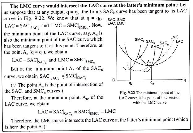
Here the minimum point of the LAC curve is A₂. Let us suppose that Ai is any point on the LAC curve to the left of the point A₂. The SAC curve that has been tangent to the LAC curve at A₁ when q = q₁, is SAC₁, Again the marginal curve to the SAQ curve is SMC₁. Therefore, at q = q₁, we obtain

LAC = SAC|_SAC1                                    (9.31)

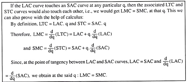
Here SAC|_SAC1 is the short-run average cost (SAC) given by the SAC₁ curve. Again, since the LAC and SAC₁ curves have been tangent to each other at the point A or at q = q₁, the LTC and STC) curves associated with them have also touched each other at q = q₁. For at q = q₁, since the LAC and the SAC₁ curves have been tangent, we obtain

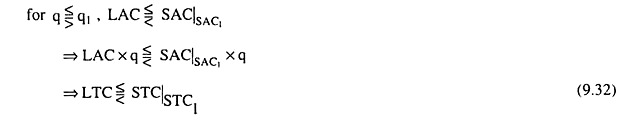
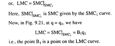
Here STC|_STC1 is the STC given by the STC, curve. (9.32) gives us that if LAC and SAC1₁ curves become tangent to each other at any q = q₁, then the LTC and STC₁ curves would also be tangent to each other at that output (i.e., q = q₁). That is, at q = q₁ we obtain the slope of the LTC curve = the slope of the STC₁ curve

We shall now consider the minimum point A₂ of the LAC curve. Since the SAC₂ curve has touched the LAC curve at this point or at q = q₂, the point A₂ will also be the minimum point of the SAC₂ curve. Therefore, the marginal curve of the SAC₂ curve, viz., the SMC₂ curve, would also pass through the point A₂. Therefore, at q = q₂, we obtain

LAC = SAC|_SAC1 = A₂q₂, and SMC₂ = A₂q₂                                  (9.33)

Again, since the LAC and the SAC₂ curves have touched each other at A₂ or at q = q₂, the LTC and STC₂ curves would also touch each other at q = q₂. Therefore, at q = q₂, we obtain the slope of the LTC curve = the slope of the STC₂ curve

or LMC = SMC|_SMC2 = A₂q₂ [by (9.33)]                                       (9.34)

From (9.33) and (9.34), we obtain at q = q₂, LAC = LMC = A₂q₂ i.e., the minimum point, A₂, of the LAC curve lies on the LMC curve also. Therefore, the LMC curve intersects the LAC curve at the latter’s minimum point.

Lastly, let us suppose, A₃ is any point on the LAC curve that lies to the right of its minimum point, A₂. We shall now consider this point. At this point, i.e., A₃, where q = q₃, the SAC curve that has touched the LAC curve is, say, SAC₃. Let us suppose that SMC and STC curves associated with SAC₃ curve are SMC₃ and STC₃, respectively. Therefore, at q = q₃, we obtain

LAC = SAC|_SAC3 = A₃q₃

Again, since the LAC and SAC₃ curves have touched each other at q = q₃, the LTC and STC₃ curves have also touched each other at q = q₃. Therefore, at q = q₃, we have slope of the LTC curve = slope of the STC₃ curve

or, LMC = SMC|_SMC3 =B₃q₃

i.e., the point B₃ is a point on the LMC curve (when q = q₃).

In our above analysis that in Fig. 9.21, when q = q₂ and q₃, we have LMC = B^, A₂q₂ and B₃q₃, respectively. That is, the LMC curve would pass through the points B_l5 A₂ and B₃. Here we have considered only three points on the LAC curve, viz., A₁, A₂ and A₃, and corresponding to these points, we have three points on the LMC curve, viz., B₁, A₂ and B₃. Similarly, we may have more such points on the LMC curve.

Therefore, if we join the points B₁, A₂ and B₃ and such other points by a curve, then that curve would be the firm’s LMC curve. Since the LTC curve of the firm is of third degree owing to economies and diseconomies of scale, its LMC curve would be a second degree or U-shaped curve. We may also note that the LMC curve would pass through the minimum point of the LAC curve.

Relation between the LMC and the LAC Curves:

Like these curves, the LMC and LAC curves are also U-shaped, although for different reasons.

If we replace SMC and SAC by LMC and LAC, we shall get the relation between the LMC and LAC curves. That is, the relation between the LMC and LAC would be the same as that between the SMC and SAC.

The main points of the relation between the LMC and LAC curves are:

(i) The LMC curve would intersect the LAC curve at the latter’s minimum point, i.e., at this minimum point we would have LMC = LAC.

(ii) To the left of this minimum point, the LMC curve would lie below the LAC curve, i.e., we would have LMC < LAC.

(iii) To the right of the minimum point of the LAC curve, the LMC curve would lie above the LAC curve, i.e., we would have LMC > LAC.

(iv) The minimum point of the LMC curve would lie to the southwest of the minimum point of the LAC curve.

It is evident that the U-shaped LAC and LMC curves of Fig. 9.23 possess these properties.

The relations between the U-shaped LMC and LAC curves give us the relative positions of these curves. The LMC curve would lie below the LAC curve to the left of the latter’s minimum point, it would intersect the LAC curve at its minimum point, and it would lie above the LAC curve to the right of the latter’s minimum point.

However, we shall see now, on the basis of the marginal-average relation, what would be the relative positions of these two curves if the LAC curve is a horizontal straight line like the one shown in Fig. 9.25. Here, at any q, and as q increases, LAC remains constant.

So from the marginal-average relation (i) given in, we would have LMC = LAC at any q. This implies that if the LAC curve is a horizontal straight line, then the LMC curve would also be the same horizontal straight line. In Fig. 9.25, we have drawn an LAC = LMC line. Here we have supposed that at any q, LAC = OC = constant.

Constant Returns to Scale (CRS) and Long-Run Cost of Production:

The constant returns to scale. In the long run, if the firm increases the quantities used of all the inputs in a certain proportion, and if, as a consequence, the quantity of output increases in the same proportion, then we say that the returns to scale are constant.

Since the prices of the inputs are assumed to remain unchanged, the firm’s output and its total cost would increase here in the same proportion as the increase in the input quantities.

This implies that the ratio between the firm’s LTC and its q is a constant which again gives us that under constant returns to scale (CRS), the firm’s LTC curve would be an upward-sloping straight line from the origin like the curve shown in Fig. 9.24. However, the LTC curve obtained here would be an envelope of the firm’s STC curves at different TFCs.

It may be noted here that owing to the law of variable proportions (LVP), the firm’s STC curves, of course, would be of the usual concave-convex shape. It may also be noted that, under constant returns to scale, there would not occur any economies or diseconomies of scale.

That is why the LTC curve would be neither concave downwards nor would it be convex downwards—it would be a straight line sloping upward towards right. Since, in the long run, all the inputs are variable, we would obtain LTC = 0 at q = 0. In other words, the LTC curve (line) would start from the origin.

In the case of constant returns to scale, the ratio of LTC to q is a constant at any q. That is why, in this case, the LAC = LTC/q would be a constant, and the LAC curve of the firm would be a horizontal straight line like the curve in Fig. 9.25.

The straight line LAC curve, of course, would be an envelope of the SAC curves, i.e., it would be made up of the points of the SAC curves, each SAC curve contributing only one point to the LAC curve.

Although the envelope LAC curve would be a horizontal straight line under constant returns to scale, there is no reason why the SAC curves would not be U-shaped, because in the short run, the LVP would be very much in force as per our assumption.

It may also be noted that, since under CRS, there would not be obtained any economies or diseconomies of scale, the LAC curve would not be downward sloping nor would it be upward sloping, i.e., it would not be U-shaped— here it would be a horizontal straight line.

Lastly, we have to remember here that, since the LAC curve would be a horizontal straight line under CRS, the firm’s LMC curve would also be the same horizontal straight line (Fig. 9.25) as the LAC curve, owing to the marginal-average relation.

Some More Points on the Relation between SAC and LAC Curves under CRS:

Under economies and diseconomies of scale, the LAC curve is obtained to be U-shaped. It is the envelope of the SAC curves.

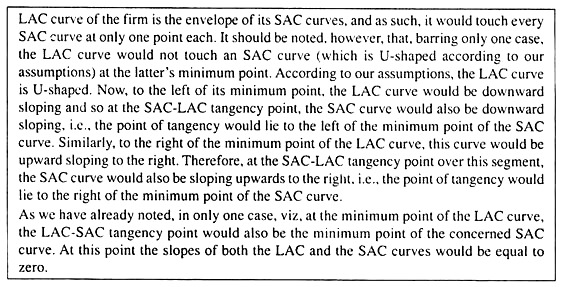
Along the downward- sloping portion of the LAC curve, the firm does not produce any output at the minimum point of a plant (SAC) curve, it produces at a point on the downward-sloping portion of a plant curve, i.e., it does not produce at the capacity (minimum average cost) point of a plant curve, rather, it produces with excess capacity.

On the other hand, along the upward-sloping portion of the LAC curve, the firm operates above capacity.

However, under CRS, the firm’s LAC curve is a horizontal straight line which can touch a U-shaped SAC curve only at the latter’s minimum point. That is, under CRS, the envelope SAC curve touches all the SAC curves at the latter curves’ minimum points. In other words, under CRS, the firm always operates at the capacity (minimum average cost) point of the plant.

We may explain this difference between the case of economies-diseconomies of scale and the CRS case in this way. At the minimum point of an SAC curve, the firm achieves the optimum proportion between the inputs.

That is why when in the long run, the firm shifts to a larger plant in order produce a larger output, it can proportionately increase the quantities of all other inputs so that the optimum proportion between the inputs would be maintained and the firm again would be producing at the minimum point of the larger plant curve, producing a proportionately higher output at a constant LAC.

Cost Elasticity, Function Coefficient and the Relationship between the Long-Run Production Function and the Long-Run Average Cost Curve:

We may now establish a very important and useful relationship between the long-run production function of the firm and its long-run average cost function. But before doing this, let us explain two new concepts—cost elasticity with respect to output and the function coefficient.

(a) Cost Elasticity w.r.t. Output:

The coefficient of cost elasticity w.r.t output (E^(C)) is defined to be the ratio of the proportionate change in the cost of production and the proportionate change in output. If the proportionate change in output is denoted by Δq/q and the proportionate change in cost is denoted by ΔC/C then we have

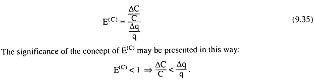
This implies that the increase in output by a certain proportion requires a less than proportionate increase in cost, or, the increase in cost by a certain proportion will lead to a more than proportionate increase in output, or, the increase in the quantities used of the inputs by a certain proportion will lead to a more than proportionate increase in output (assuming that the prices of the inputs remain constant), which implies that the returns to scale are increasing. It is, therefore, obtained that if cost is relatively inelastic w.r.t output (E^(C) < 1), returns to scale will be increasing.

In the same way we would obtain that, if cost is relatively elastic w.r.t. output (E^(C) > 1), returns to scale will be decreasing. Lastly, if cost is unitary elastic w.r.t output (E^(C) = 1), an increase in output by a certain proportion will require an increase in cost by the same proportion, or, an increase in the usage of inputs by a certain proportion will lead to an increase in output by the same proportion, i.e., the returns to scale will be constant.

(b) The Function Coefficient:

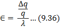
The function coefficient (or, the elasticity of the production function) is the ratio of the proportionate change in output and the proportionate change in the inputs. Let us suppose that all the inputs used by the firm are increased by a certain proportion, λ, and, as a result, the proportionate increase in output is obtained to be Δq/q. Then, by definition, the function coefficient (ԑ) would be

It follows from (9.36) that

(i) if the function coefficient is unitary (ԑ =1), then the change in the inputs by a certain proportion would lead to a change in output by the same proportion, and we say that the returns to scale are constant,

(ii) If e < 1, then the proportionate change in output is less than the proportionate change in inputs, and we say that the returns to scale are decreasing, and

(iii) if ԑ > 1, then the proportionate change in output is greater than the proportionate change in inputs, we say that the returns to scale are increasing.

Let us now suppose that the production function of the firm is

q = f(x, y)                          (9.37)

Then for small change in x and y by Δx and Δy, the change in output would be

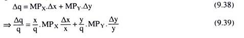
Let us now suppose that x and y increases by the same proportion 1, i.e., Δx/x = Δy/y = λ, then we have from (9.39),

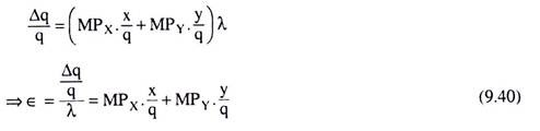
Since q/x is the average product of input X (i.e., AP_X) and q/y is the average product of input Y (i.e., AP_Y), we may write (9.40) as

The result given by (9.41) is easily understood if X is the only factor. Then the function coefficient would be the ratio of MP_X and AP_X. Now, by definition, AP_X is the average product of all the units of X that have been already employed, and MP_X is the output produced by the marginal unit or an additional unit of X.

It follows then, and we may easily understand this, that if ϵ > 1, or, MP_X > AP_X (assuming X to be the only input used by the firm), then the productivity of the marginal unit is greater than that of all the previous units, which implies that the firm is becoming more productive as the quantity used of input X and the quantity of output expand, which, in turn, implies that the returns to scale are increasing.

Conversely, if ϵ < 1, or, MP_X < AP_X, the firm would become less productive as the quantity used of input X and the quantity of output expand, i.e., there would be decreasing returns to scale. Lastly, if ϵ = 1, or, MP_X = AP_X, the firm would remain equally productive as the quantity of X and that of the output expand, and, in this case, the returns to scale would be constant.

(c) Relationship between Long-Run Production Function and Long-Run Average Cost Curve:

Let us now suppose that the prices of inputs X and Y are P_X and P_Y, respectively. We may now write (9.40) as

As we know, the first-order condition for constrained cost-minimisation is

From equation (9.42) and (9.43) we have

Finally, in this two-input case, the firm’s total cost (C) is given by

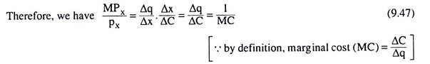
Now, since the average cost (AC) is defined as C/q, from (9.44) and (9.45) we have:

Let us now note that MP_X is Δx/Δy and p_X is simply the rate of change of cost w.r.t. x, i.e., p_X = ΔC/Δx

Therefore, from (9.46) and (9.47), we have

Relation (9.48) has some important implications. Let us analyse them. ϵ > 1 implies increasing returns to scale, i.e., the increase in the usage of inputs by a certain proportion gives rise to an increase in output by a large proportion.

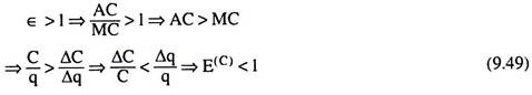
That is, here, ԑ > 1 implies E^(C) < 1, i.e., an increase in output by a certain proportion would require an increase in cost by a smaller proportion, which again implies that average cost declines as output increases. What we have obtained, therefore, is that over the range in which the long- run production function exhibits increasing returns to scale (g >1), the long-run average cost curve declines.

Conversely, we would obtain:

ԑ < 1 => E^(C) > 1 (9.50)

That is, over the range in which the long-run production function exhibits decreasing returns to scale (ԑ < 1), an increase in output by a certain proportion would require a more than proportionate increase in cost (E^(C) >1), which implies, average cost would increase as output increases and the long-run average cost curve would be upward sloping.

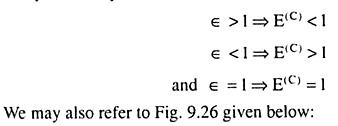
Lastly, we would obtain:

ԑ = 1 => E^(C) = 1                                              (9.51)

That is, if over some range, the long-run production function exhibits constant returns to scale (ϵ =1), an increase in output by a certain proportion would require a proportionate increase in cost (E^(C) = 1), i.e., the average cost would remain unchanged as output increases, and the long-run average cost curve would be horizontal.

In the above analysis, we have obtained, therefore, that the LAC curve slopes downwards or upwards or become horizontal according as the returns to scale are increasing, decreasing or constant.

Let us not also the following relations between the function coefficient (ԑ) and the cost elasticity w.r.t. output (E^(C)):