The following points highlight the top three aspects of cost estimation. The aspects are: 1. Short-Run Cost Estimation 2. Long run Cost Estimation 3. Cost Forecasting.
Aspect # 1. Short-Run Cost Estimation:
The techniques of short-run cost estimation are the following:
a) Simple Extrapolation:
The term ‘extrapolation’ refers to the assignment of value to a sequence of results, beyond the range of these actually given or determined. Unless we have a known functional relation between the results (in which case extrapolation is merely the calculation of additional values), any process of extrapolation assumes “that a relation is maintained beyond the range and domain for which it is actually established.”
The simplest method of short-run cost estimation is “probably to ascertain the present level of marginal or average variable costs and extrapolate this backward or forward to other output levels.” Most business managers believe that both marginal and average variable costs of their plants are constant over a range of output levels surrounding the current output level.
ADVERTISEMENTS:
This implies that constant re– turns to the variable factors occur over this range of output. If this constant efficiency situation actually exists in the short-run production process, then the simple extrapolation method of cost estimation gives accurate results.
However, in reality, the short run production function exhibits diminishing returns to variable factor, i.e., marginal costs rise after a certain stage of the production process. Therefore, if marginal costs are simply believed to remain constant, when, in fact, they are increasing with every additional unit of output, the simple extrapolation method may give erroneous results and thus cause poor decisions to be made.
b) Gradient Analysis:
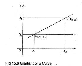
Gradient is the measure of the steepness of a slope, expressed in the Cartesian plane as the ratio between differences of ordinates and abscissae. Then the gradient of the line PQ joining P(x1, y1) to Q(x2,y2) is given by y2-y1/x2– x1.
It is then equal to tan 8, where 6 is the angle of slope as in Fig. 15.6.
Since output of a business firm does fluctuate from period to period, it is possible to find two or more cost/output observations, in which case one can conduct gradient analysis. It may be noted that the gradient of each cost category is the rate at which that cost category changes with changes in the level of output.
If we exclude those cost changes which are not the result of changes in the output level (e.g., an increase in annual licence fee), we can estimate the marginal cost (per unit) over range of output under observation on the basis of the sum of the gradients.
In fact, three or more observations permit gradient analysis to accurately estimate the change in marginal costs with changes in output levels. If we have various cost/output observations, we can make use of the technique of regression analysis for short-run cost estimation.
(c) Time-Series Regression Analysis:
If we have a set of cost-output observations, we can apply regression analysis to estimate the functional dependence of costs upon the volume of output and thus arrive at an estimate of the marginal cost. If our object is to estimate the cost function for a particular firm, we must make use of time- series data from the firm.
ADVERTISEMENTS:
However, the problem with time-series data is that if, over the observation period, some factors have changed, the results of regression analysis will be less reliable. Changes in factor prices, for instance, due to inflation or market forces and/or factor productivities due to technological change and improvement in efficiency of labour may make regression analysis irrelevant.
To eliminate these problems to the maximum possible extent the cost data should be appropriately deflated by the price index, and time should be included as an independent variable in the regression equation. This will make it possible to include any trend in the relative prices or productivities in the co-efficient of the time variable.
One major drawback of this method is that it is subject to problems of measurement error. As E. J. Douglas has commented: “The cost data should include all costs that are caused by a particular output level, whether or not they are yet paid for.”
He has cited the example of management expense which should be expected to- vary with the rate of output, but it may be delayed until it is more convenient to close down certain sectors of the plant or facilities for maintenance purposes.
Hence the cost that is incurred in an earlier period is recorded in a later period and is thus likely to understate the previous cost level and overstate the later cost level. True enough, “our cost/output observations should be the result of considerable fluctuations of output over a short period of time with no cost/output matching problems.”
Moreover, the choice of the functional form of the regression equation has major implications for the estimate of the marginal cost curve which will be indicated by the regression analysis. Three functional forms of costs considered earlier in this chapter may now be considered.
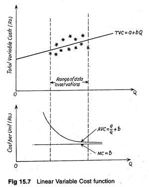
If the short-run cost function is linear, i.e., if we specify that total variable cost is a linear function of output such as TVC = a + bQ, the marginal cost estimation generated by the regression analysis will be the parameter b. It is because marginal cost is the total variable cost function with respect to output changes.
In Fig. 15.7 we show, for a given set of data (based on various observations), the consequent average variable cost and marginal cost curves that would be generated by regression analysis in this case. In this case, the AVC will decline to approach the MC curve asymptotically.
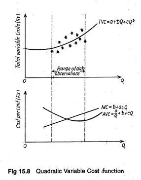
Alternatively, for the same set of data, we can use a quadratic cost function such as TVC = a + bQ + cQ2. In this case, the marginal cost will rise as a constant function of output. This is shown in Fig. 15.8 where the hypothesized quadratic relationship is superimposed upon the same data observations, with the resultant AVC and MC curves illustrated in the bottom half of the diagram.
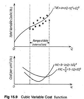
Finally, if we specify the functional form to be cubic, such as TVC = a -bQ- cQ2 + dQ3, the estimate of MC generated by regression analysis will be curvilinear and will increase as the sequence of the output level. Fig. 15.9 illustrates such a cost- output relationship. We can alternatively specify the functional relationship to be a power function.
The choice of the functional form depends upon the degree of accuracy to be achieved. Since the results of regression analysis are used for decision-making purposes, one must ensure that the marginal and average cost curves generated are the most accurate representations of the cost/output relationships.
ADVERTISEMENTS:
By plotting the total variable cost data against output, it may be possible to ascertain that one of the above three functional forms best represents the apparent relationship existing between the two variables and piece of information may be used for decision-making.
d) The Engineering Technique:
An alternative method of cost estimation is known as the engineering technique. It simply consists of developing the relation that exists between the inputs and the output (on the basis of the physical production function) and attaching cost values to the inputs in order to obtain a TVC figure for each level of output.
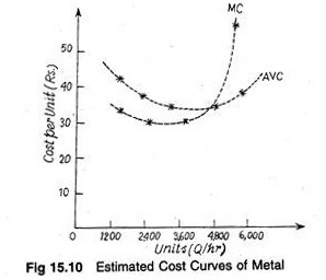
We then have to calculate, or test for each level of output, the amount of each of the variable factors necessary to produce that level of output. By attaching costs to these variable factors, it is possible subsequently to calculate (estimate) the TVC for each level of output and the corresponding AVC and MC.
In Fig. 15.10, we draw average and marginal cost curves on the basis of actual data. Interpolating through these observations it is possible to estimate marginal and average costs by using the engineering technique.
ADVERTISEMENTS:
Moreover, it is also possible to determine incremental costs associated with any decision to increase or decrease output levels on the basis of the variable costs as calculated by one or a combination of the above methods, after making an allowance for any opportunity costs that are involved and any incremental fixed costs that may be necessitated.
It is necessary to calculate incremental fixed costs on the basis of the knowledge of the production capacity of the fixed factors involved. This, in its turn, may require an engineering-type investigation of the output capacities of particular fixed facilities.
Studies of Short-run Cost Behaviour:
ADVERTISEMENTS:
Numerous empirical estimates of short-run cost have led to the conclusion that marginal cost tends to be constant in the operating range of the firms studied.
Hence, it follows that AVC is constant at the same level (or is asymptotically approaching that level) and declining due to the influence of declining AFC. ATC will also decline. In other words, in most cases, a linear TVC function provides the best fit to the data observations.
Aspect # 2. Long Run Cost Estimation:
When suitable actual cost-output data are available, statistical methods similar to those used in short-run cost factors can be employed in analysing long-run behaviour of cost. The method most commonly used for the purpose is cross-section method. A sample of inter-firm differences is called a cross- section sample.
In a cross-section model, we may have the same sort of cost function but now the data relate to different units of observation at a given point in time. Two other techniques used for long term cost estimation are: the engineering technique and the survivor technique.
a) Cross-Section Method:
The long-run cost function can be estimated using either time-series cost-output data collected on a plant (or firm) whose size has been variable over time, or cross-sectional cost-output data collected on a sample of plants (firms) of different sizes at a particular point in time.
Both the approaches require certain assumptions about technological and operating conditions to be made in order to arrive at valid estimates of the long run cost function.
ADVERTISEMENTS:
When one uses time-series cost-output data one encounters the usual problems of holding constant all other factors (except output) that affect costs. In order to estimate the long-run cost function from time-series data, one must make use of observation taken over a fairly long period of time, usually a number of years, to allow for sufficient variation in plant size.
However, due to technological change and development of new products in the product line, the long-run cost curve may shift over time.
If it is not possible to hold the effects of such changes constant, the cost-output data will be measuring points on different long-run cost functions rather than on the same function. Moreover, using time-series requires that costs be deflated to reflect changes in prices over long periods of time.
The above reasons justify the use of the cross- sectional data in estimating long run cost functions. Data observations from various plants at a fixed time period may be analysed using the technique of regression analysis. Thus the researcher should collect pairs of data observations relating the output level, to the total cost of obtaining the output level in each plant, for a very short period of time.
Measures should be taken in such as a way as to avoid errors of measurement relating either to the actual level or rate of output in that period, or to the actual level of costs that should be associated with the level of output in each plant observed.
There is also need to specify the functional form of the equation and the problem here is the same as in the case of short-run cost estimation. We have to choose the functional form that best fits the data observations subject to each variable determining cost being significant at an acceptable level.
ADVERTISEMENTS:
The behaviour of long run average cost largely depends on economies and diseconomies of scale. Therefore, the cubic function which is consistent with economies and diseconomies of plant size would be most appropriate. If, however, a linear function best fits the data, we may be driven to the conclusion that increasing returns to plant size prevail over the range of data observations.
Finally, if a power function best fits the data, the numerical value of the exponent to the output variable will indicate whether returns to plant size are increasing (if it is less than one), or constant (if equal to one), or decreasing (if it is greater than one).
In addition to this problem which arises in a short-run cost analysis, further difficulties of a conceptual nature are also encountered in estimating the long-run cost-output relationship by statistical methods.
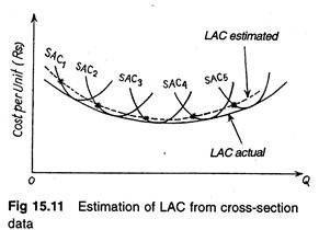
One major problem with cross-section data is that the observations collected may not be points on the long-run average cost curve at all. This is shown in Fig. 15.11. It depicts the five short run average cost curves (SAC1, SAC2 etc.) of a firm. Each curve corresponds to a specific plant. The estimated output/cost values are shown by the point on each short run cost curve marked by an asterisk.
This small piece of information suggests that the above analysis has over-estimated the presence of economies and diseconomies of plant size in this particular case. It is because of the fact that the observation points for each plant were not points of tangency with the actual long-run cost curve.
ADVERTISEMENTS:
The second problem that may arise with cross- section data is that various plants may be operating in different areas or under different economic and non-economic environments.
As a result, there may be differences in factor prices and factory productivities among the plants. If this problem exists, there may be cost differences among plants due to the two above factors and regression analysis may fail to give accurate results.
b) The Survival Principle:
If there are economies of scale that a firm fails to exploit, long run average cost of production will be higher than of competing firms; the firm will be too small for efficient operation and must either grow or perish.
Many people believe that production by larger firms will be less costly on average than by small firms. Even if a firm has to be large enough to exploit the economies of scale that are available, bigger plants may encounter diseconomies of scale and be forced to reduce the scope of their operations or sink.
If firms (production facilities) of a particular size tend to exist in an industry, this is considered to be a good evidence of the requisites size that is most efficient. This is known as the survival principle put forward by G. Stigler in 1958. Some economists have used this principle to determine the most efficient scale of operations for a particular industry.
Stigler has devised a test for the presence or absence of economies or diseconomies of plant size in specific industries which is based upon the survival principle stated above. The implication is that the most efficient firms will be able to survive in the long run and even increase their market share, while the less efficient ones will tend to become less important in that industry with the passage of time.
The survival principle is a method of determining the optimum size (or range of sizes) of firms within an industry. Stigler’s procedure was to classify the firms in an industry by size and calculating the share of industry output coming from each size class over time.
If the share of industry output of a given class tends to decline over time, then this size class is presumed to be relatively inefficient and to have higher LACs. On the contrary, an increasing share of industry output over time indicates that the size class is relatively efficient and has lower LACs.
The rationale of this approach is that the forces of competition will tend to eliminate relatively inefficient firms, leaving only efficient (low-cost) firms to survive in the long run. According to Stigler, “An efficient size of firm is one that meets any and all problems the entrepreneur actually faces: strained labour relations, rapid innovation, government regulation, unstable foreign markets and what not.”
Merits:
Two things may be said in favour of the survivor technique. Firstly, it is more direct and simpler to apply than are alternative techniques for examining economies of scale. Secondly, it avoids the accounting-cost allocation and resource valuation problems associated with statistical methods and the hypothetical aspects of the engineering method of cost estimation.
Limitations:
However, this method has two major limitations as well. Firstly, it does not utilize actual cost data in the analysis. Thus, it is not possible to assess the magnitude of the cost differentials among firms of differing size and efficiency. Secondly, due to legal factors, the LAC curve derived by this technique may be distorted and may fail to measure the cost curve postulated in traditional economics.
For example, in India, the MRTP Act (1969) discourages larger firms even though economies of scale are likely to be stronger beyond present firm sizes of the so-called MRTP companies.
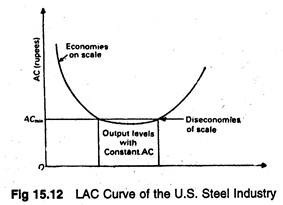
Stigler’s test of the US steel industry for the years 1930 and 1951 indicated that both the smallest and largest firms suffered a decline in their market share. The firms of intermediate size grew or maintained their shares of industry output over this period and hence appeared to be operating at the optimum sizes of plant.
Thus, the survival principles infer a LAC curve that slopes downward at first, is constant over a wide range of output (in the intermediate stage) and then slopes upward at relatively higher output levels. In other words, there are typically substantial ranges of output for which LAC is roughly constant, as depicted in the middle of the LRAC curve in Fig. 15.12.
c) The Engineering Technique:
The engineering technique used in short-run cost functions may also be applied to several plants of different sizes, at the same point in time, to arrive at an estimate of the long-run cost function.
This approach needs a knowledge of production facilities and technology (such as speed of machines, labour productivity and physical input-output transformation relationships) to determine the most efficient (lowest average cost) combination of resources (capital, labour, materials, etc.) to produce various levels of output.
It may be recalled that in the context of short- run cost estimation, the engineering technique was used to find the cost curves of a particular firm at’ a fixed point of time. If the same exercise is carried out with other plants that are available, one would be able to trace out a series of short-run cost curves that are available to the firm at a definite time period.
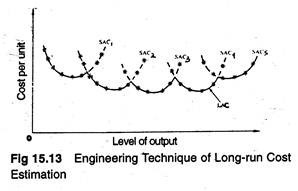
Fig. 15.13 shows a hypothetical situation in which five different sizes of plants have been observed and the SAC curve of each has been derived by the engineering technique. The envelope of the SAC curves is the LAC curve.
One can infer from Fig. 15.13 that initially there are economies of plant size as one moves from the first plant to the second plant. This stage is followed by relatively constant returns to plant size as one progresses to the third and fourth plant, and decreasing returns to plant size with the largest plant available.
Merits:
The engineering method has three major advantages over statistical methods. Firstly, it is generally much easier with the engineering method to hold constant such factors as prices of factors, product mix and production efficiency (technological progress).
This enables us to isolate the effects of changes in output on costs. Secondly, the long-run cost function obtained by the engineering method is based on current technology whereas the function obtained by the statistical method is based on a mix of old and current technology. Finally, the engineering methods makes it possible to avoid some of the accounting problems normally encountered when using the statistical approach.
Defects:
However, the major disadvantage of the method is that it deals only with the technical aspects of the production process or plant. It completely ignores various other aspects affecting cost behaviour such as “the management and entrepreneurial aspects, such as recruiting and training workers, marketing the product(s), financing the operation and administering the organisation.”
Haldi and Whitcomb made a study to isolate the various source of scale economies within the plant. They collected data on the cost of individual units of equipment, the initial investment in plant and equipment, and operating costs (namely labour, raw materials, and utilities).
They found that “…in many basic industries such as petroleum refining, primary metals and electric power, economies of scale are found up to very large plant sizes (often the largest built or contemplated). These economies occurs mostly in the initial investment cost and in operating labour cost, with no significant economies observed in raw material cost.”
Long-run Cost Estimation Studies:
Various empirical studies have been made of the long-run cost function. J. Johnson developed long- run cost functions using both time-series and cross- section data. In the time-series analysis, he fitted a cubic cost function with a linear trend variable to each of 23 firms whose capital equipment had varied over the period 1928-1947. The cubic term was not found to be statistically significant.
Most studies of long-rim cost functions have revealed that the long-run average cost curve tended to be L-shaped, not U-shaped.
This signified economies of plant size at relatively low levels of output, followed by an extended range of constant returns to plant size with no common tendency for per unit costs to rise at higher output. Statistical studies of long-run cost behaviour fail to provide sufficient evidence on significant diseconomies of scale (size).
Managerial uses of Empirical Cost Functions:
Various important managerial decisions are based on estimates of cost curves such as short- run choices of rates of output and prices, and long- run decisions about numbers, sizes and locations of plants.
Pricing and output decisions are perhaps the most important for a profit-maximising firm. Such decisions must be based on reliable estimates of short-run cost functions.
Capital investment decisions such as plant construction or expansion are long-term decisions and are usually based on estimates of long-run cost functions. Long-run cost functions enable progressive organisations to determine whether or not to make the investment, and what should be optimum size of the plant under the present conditions. Decisions on plant size are largely based on an accurate estimate of demand.
However, investment decision are most complex because demand can shift over time. Moreover, the structure of factors affecting cost may also be expected to shift. These factors make it advisable to build or expand plants in substantial increments of capacity.
It is important to note that past production and cost relationships may not always be relevant to decisions about future investments in plant and equipment.
Empirical (statistical) estimates may require adjustments to reflect changes in future prices, input combinations, nature of the product, product mix, scale of output, scale of plant, the nature of the conversion process (i.e., conversion of inputs into output) and so forth; all these are expected to effect future costs. Costs of future periods may not behave in the same way as that in the past.
Aspect # 3. Cost Forecasting:
One of the most important problems before a professional manager is to surmise what the cost of production is going to be in the future. Cost forecasting, therefore, is an important topic in managerial economics. It must be emphasised at the very outset that cost forecasting has to be differentiated from what is known as cost estimation.
The short and long run cost functions that we have discussed above can be statistically estimated. It is this process of statistical determination of the cost-output relationship that is referred to as cost estimation. As we have noted, both short and long-run cost functions refer to the cost of production of the company at various levels of output.
The only difference between these two cost functions is that, in the short- run function, the plant size is taken to be fixed while in the long-run function, it is considered to be variable. It is to be specifically noted that the long-run cost function does not refer to cost of production in the future.
It tells us what the cost of production at alternative levels of output would be today if each level of output could be produced at an optimal plant size. Cost forecasting, on the other hand, refers explicitly to the future. The question here is: what would be the cost of production (of, say, a specified level of output) in the future?
We do not wish to imply that the problem of cost estimation is not important. Indeed, as we have emphasised throughout our discussion above, a company must know its cost function before it can hope to take optimal decisions regarding the level of output to be produced and the size of the plant to be built.
However, we have already formed a fairly comprehensive idea about estimation techniques in general in course of the discussion of demand analysis.
In particular, we are now familiar with the most important statistical estimation technique, viz., regression analysis. Statistical cost functions can be estimated by applying these techniques on the theoretical models of cost functions. Entering into a detailed discussion of cost estimation will, therefore, involve a large dose of repetition. We have, therefore, decided to concentrate on the problem of cost forecasting.
We have seen above that the cost function is derived from two types of information – the production function and the prices of inputs. If these primary information remain unchanged, the cost function will be totally unchanged.
It will be exactly the same as it is today. The problem of cost forecasting arises because neither the production function nor the prices of the inputs would necessarily remain unchanged in the future.
The production function, it may be recalled, is a technological relationship between output and inputs. If productivity of the inputs changes (i.e., if from the same amounts of inputs we can extract a different level of output) the production function will change.
The prices of inputs used by the company, on the other hand, would change in pace with the general level of factor prices (or, more generally, with the process of inflation or deflation) in the economy. Future changes in factor productivities and in factor prices are, therefore, the focus of attention in cost forecasting. We shall deal briefly with these two aspects of cost forecasting separately.
