Division of Classical Macroeconomics (With Diagram) | The Classical Model

The following points highlight the Division of Classical Macroeconomics for Analytical Convenience.The two Divisions are: (A) Equilibrium Output and Employment (B) Money, Prices and Interest.

(A) The Classical Theory of Output and Employment (the Real Sector):

i. Aggregate Production Function:

A basic component of the classical model of the real sector of the economy is the aggregate production function, which is expressed as:

Y = F (K, L) … (1)

where Y is output, K is fixed stock of capital (plant and equipment) and L is the quantity of homogenous labour. In the short run, the capital stock (K = K), the size of the population and the state of technology are all assumed to remain fixed (constant).

So output varies with changes in the usage of labour, the supply of which depends on the fixed population. So Y depends on — or is a function of — L alone as shown by equation (1).

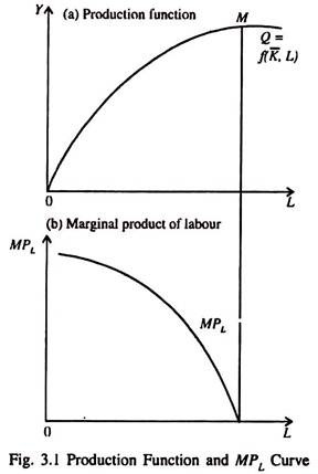
In Fig. 3.1(a) the production function shows how output y responds to an increasing application of labour (CL), which is the only variable factor of production. Fig. 3.1(b) shows the marginal product of labour (the addition to Y made by every extra unit of labour, the quantity of other inputs remaining the same).

MP_L falls due to diminishing returns — every extra worker makes less and less contribution to total product. This means that the marginal product of each worker is less than that of the previous worker.

The short-run production function shown in Fig. 3.1(a) is a technological relationship between the level of output for each level of labour input (employment), when capital stock, level of technology and skill-level of workers remain the same.

Classical econo­mists assumed that the level of employment would be determined by the forces of demand and supply in the labour market. It is to this important point that we turn now.

Employment:

In the classical model, where firms seek to maximise profit and workers try to optimise (maximise) their wage income the labour market clears automatically. There are no barriers to the adjustment of money wages.

i. Labour Demand:

Since in the short run, output is varied solely by changing the labour input, the choice of the level of output and quantity of the labour input are one decision.

Since there is perfect competition in both labour and product markets, a profit-maximising firm will reach the point of optimal purchase of labour by equating the marginal cost of producing a unit of output to the marginal revenue product — which is the extra revenue obtained by selling one extra unit of output.

Under perfect competition, since MR = P. MRP = MR x MP_L. Moreover, since labour is the only variable factor of production, the marginal cost of each unit of output is the marginal labour cost. Marginal labour cost equals the money wage divided by the number of units of output produced by one extra worker. Thus marginal cost for the ith firm (MC) is equal to the money wage (WO divided by the marginal product of labour for that firm (MP):

MC_i = W/MP_Li … (2)

The condition for short-run profit maximisation in a purely competitive market is

P = MC_i … (2a)

Substituting the expression for marginal cost (MC) from (2) into (2a) shows that the short- run profit-maximising condition for the firm buying labour from a competitive market:

P = W/MP_Li … (3)

In the labour market, firms maximise profit by hiring labour services up to the point where MRP_L = MC_L, which is the marginal cost of labour (or marginal wage). In this case, we get from equation (3) the following profit-maximising condition, i.e., condition for the optimum purchase of labour:

P.MP, = W/MP_LI. MP_Li (by multiplying both sides of equation (3) by MP_Li) or, MP_Li = W/ P (dividing both sides by P)

or, W/P = MP_Li … (4)

This means that a profit-maximising firm will hire labour up to the point where the additional output produced by employing one extra worker (MP_L ) is just equal to the real wage (W/P) paid to hire that worker. Now by multiplying both sides of equation (4) by P we get:

W = MP_Li.P …(5)

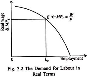
This is just an expression of the profit-maximising condition in terms of money wage. The condition for profit-maximisation, in real terms, is met in Fig. 3.2 at point E where the real wage (W/P) is equal to the marginal product of labour (MP_L).

The marginal product curve of labour is the firm’s demand curve for labour in a competitive market. In the classical model, labour demand varies inversely with the level of real wage.

The labour demand curve is downward sloping due to the operation of the law of diminishing returns. In short, the higher the real wage, the lower the level of labour input that will equate the real wage to the MP_V The demand curve for labour for the economy as a whole is the horizontal sum of the labour demand curves of all the firms.

For each real wage, this curve will indicate the total quantity of labour demanded by all the firms in the economy.

This aggregate labour demand function (L^d) may be expressed as

The negative sign within the bracket indicates that an increase in the real wage lowers labour demand.

ii. Labour Supply:

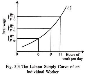
In Fig. 3.3 we show the supply curve of labour of an individual worker (j). As the real wage rate goes up, an individual worker puts more effort.

The labour supply equation is expressed as:

The positive sign indicates that L_s varies directly with (W/P). Although the supply curve of an individual worker may be backward bending (due to leisure preference), the aggre­gate supply curve of labour is upward sloping (since the substitution effect of a rise in the wage rate out-weighs the income effect).

So, in the classical economy, labour supply depends on real wage, not on money (nominal) wage. This means that if either the money wage or price (or both) change, the number of hours worked is determined by moving along the labour supply curve.

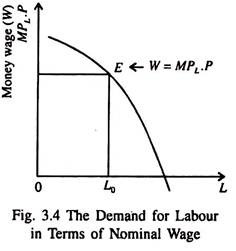
It is also possible to show the demand for labour in terms of nominal wage. In Fig. 3.4 a profit-maximising firm will hire labour up to the point (E) where the money wage is equated with the marginal product of labour times the price of the product (W = MP_L.P).

Two assumptions about the classical labour market are: (1) perfectly flexible prices and wages and (2) perfect information on the part of buyers and sellers of labour about market prices. This means that both work­ers and employees (firms) know the command over commodities, i.e., real wage (W/P) that will result from a given money wage (W).

These two assumptions are necessary for the classical equilibrium theory of em­ployment and output.

Equilibrium Output and Employment:

The three basic relationships of classical model are: Y = F (K, L) (aggregate production function)

where L^d = f (W/P) (labour demand schedule)

L^d = g (W/P) (labour supply schedule) These relationships together with the equilibrium condition for the labour market

L^s = L^d …(8)

determine output, employment and real wage in the classical system. AH three are endogenous variables, i.e., determined within the model.

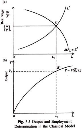
Equilibrium in the classical model is illustrated in Fig. 3.5. Part (a) shows labour market equilibrium at real wage (W/P) at equilibrium point E, corresponding to equa­tion (8). In the aggregate, labour supply equals labour demand: L^d = L^s. The equi­librium level of employment is L₀. Corre­sponding to this level of employment, we determine in part (b) equilibrium aggregate output, Y₀, at point E’.

Thus we see that in the classical model the factors that determine output and em­ployment also determine the positions of the labour supply and demand curve as also the position of the aggregate production function.

In the classical model, the level of output and employment are determined by all the variables that affect the supply side of the market for output — the amount firms choose to produce.

i. Labour Market Equilibrium in Terms of Money Wage:

It is also possible to show labour market equilibrium in the classical model in terms of nominal wage. The quantity of labour that will be demanded by firms at any money wage depends on the price level.

From equation (5) W = MP_Li .P we get: W/P = MP_Li … (9)

Given the money wage, a profit-maximising firm will choose the level of employment at which

W = MP_L.P

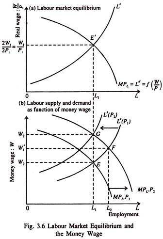
This relationship is illustrated in Fig. 3.6. Part (a) shows the how the equilibrium level of employment is determined (at L₁) where L^d = L^s. In part (b), we plot labour supply and
labour demand as functions of money wage. Since the money wage is shown on the vertical axis, a rise (fall) in price will lead to a fall in real wage and will shift the labour supply curve to the left (right).

Starting from equilibrium point E, a rise in the price level (from P₁ to P₂) will shift the demand curve for labour to the right (from MP_L.P₁ to MP_L.P₂) since the firm will earn more revenue by selling the output of each worker. So the firm will be induced to produce and sell more output at a higher price and so employ more workers.

So labour market equilibrium will now be at point F in part (b). However, at this point, the rise in price (Δ P = P₂ – P₁) is higher than the rise in wage (Δ = W – W₁). This means that the real wage has fallen. So workers will work less at each money wage because price has increased faster than money wage, leading to a fall in real wage.

Conse­quently the labour supply curve shifts to the left from L^s (P₂) so as to equalise the change in money wage to the change in price. The final equilibrium in the labour market occurs at point G, where Δ P = AW. This means that since the money wage rises (from W₁ to W₂) pro­portionately with the price level W₂ / P₂= W₁/P₂, i.e., the real wage has not changed.

In response to a price change, the demand and supply curves of labour shift simultaneously and proportionately, but in opposite directions. The supply curve of labour shifts to the left exactly by the amount by which the demand curve for labour shifts to the right. The end result is that both real wage and the level of employment remain unchanged. Here

2W₁/2P₁ = W₁/P₁ and L = L₁

ii. Aggregate Supply Function:

Perhaps the most notable feature of the classical model is the supply-determined nature of real output and employment. By using the information given in Fig. 3.6, we can construct the classical aggregate supply function, which brings into focus the supply-determined nature of output in the model.

The aggregate supply curve shows the total output all firms will supply at each price level (which is a weighted average of all prices). It shows the output forthcoming at each price level.

It is interesting to note that the supply curve of an individual firm is upward sloping, but the aggregate supply curve is a vertical straight line. The reason is easy to find out. Under perfect competition (in the product market) a firm maximises profit by equalising marginal cost with the price of the product, i.e., W/MP_Li = P

or, MP_Li = W/P …(11)

i.e., the marginal product equals the real wage. Since the labour market is also perfect, an individual firm is a price taker, i.e., it takes the money wage as given (fixed) while deciding on the optimal output to supply and, therefore, the quantity of labour to hire. Since money wage is assumed to remain fixed, the (output) supply curve of an individual firm is positively sloped. Higher prices imply lower real wages.

Consequently the firm demands more labour and produces more output. But for the economy as a whole money wages will vary, as output and demand for labour rise or fall, in order to maintain equilibrium in the labour market. Thus, while constructing aggregate supply curve, we have to take note of this possibility.

iii. Construction of the AS Curve:

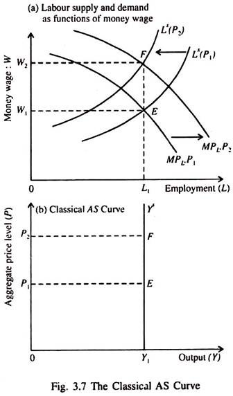
In Fig. 3.7, we derive the classical AS curve. In part (a) at equilibrium point E, the price level is P₁, the money wage is W₁ and employment L₁. When the price level rises to P₂, equilibrium is at point F, where the money wage is W₂ but the level of employment remains constant. This means that in the classical model output is not a function of price.

Any change in the price level leads to proportional change in the money wage, leaving the real wage unchanged. As a result there is no change in equilibrium employment and, so, in aggregate output. This is why the classical aggregate supply (AS) curve is a vertical straight line.

This reflects the fact that higher values of the price level require proportionately higher levels of the money wage for maintaining equilibrium in the labour market.

The real wage, employment, and, therefore, level of output, remain the same at P₁ and P₂. The vertical aggregate supply curve im­plies that output (Y) is completely sup­ply-determined in the classical model. Output is determined by the relationship of the labour market with the aggregate production function.

For output to be in equilibrium the economy must be on the aggregate supply curve; output must be Y₁. Thus, in the classical model, at equilibrium, three key variables are determined simultaneously—real output, real wage and the level of employment.

iv. Factors Influencing Output:

Since in the classical model output and employment are supply-determined, the level of aggregate demand will have no effect on output. So all such factors which affect aggregate demand as the quantity of money, level of government spending, the level of demand for investment goods by business firms have no role in determining output and employment.

To the extent that taxes affect aggregate demand, they will not affect output or employment. But changes in tax rates do affect output and employment because they have incentive or supply-side effects.

v. Change in Aggregate Output:

In the classical system, changes in the price level do not affect any of the real variables in the system the real wage, the level of employment, or real output. However, an increase in capital stock will change output in the model by affecting the aggregate production function and labour market.

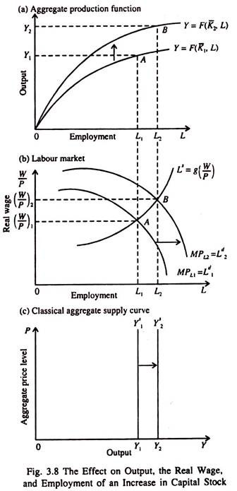
In Fig. 3.8 the initial equilibrium is at point E on the production function, labour market and with the AS curve Y_s, with equilibrium levels of real wage (W/P), employment L, and output, Y₁. Now, due to purchase of new capital goods which embody higher levels of technology the marginal product of each worker increases. Consequently the production function shifts because the output of each additional worker is higher.

The new production function Is Y = F(K̅₂, L). Due to an increase in the MP_L, the demand for labour increases (at constant product price). As the demand curve for labour shifts to the right, now F is the new point of labour market equilibrium. As real wage rise, workers are now willing to put more effort.

Consequently the equilibrium employment increases from L₁ to L₂. This, in its turn, leads to an increase in aggregate output from Y₁, to Y₂ through the production function. The end result is a rightward shift of the aggregate supply curve from Y¹_S to Y²_S, which leads to an increase in output from Y₁ to Y₂.

(B) The Classical Theory of Money, Interest and Prices:

The classical theory of the price level, or the classical theory of aggregate demand, is a hybrid that adds a theory of money to the classical theory of aggregate supply.

In order to analyse the classical theory of determination of the aggregate (general) price level we have to refer to the demand side of the model. The objective is to determine the aggregate price level.

i. The Quantity Theory of Money:

In the classical model the price level is determined by money supply. So money plays the all-important role in aggregate price level determination. It has no role in aggregate output determination. In the classical theory, the quantity of money determines the level of aggregate demand, which, in its turn, determines the price level.

The classical theory of the price level is sometimes called the quantity theory of money or the classical theory of aggregate demand. It was developed at the end of the 19th century and the beginning of the 20th century, although early versions of the theory can be found in the work of David Hume, an 18th-century Scottish economist.

ii. The Equation of Exchange:

The relation between the money supply and the aggregate price level was first studied in a systematic way by Irving Fisher in 1911. Fisher started with a simple equation, known as the equation of exchange. It is an identity relating the volume of transactions at current prices to the supply of money times the rate of money turnover (i.e., turnover rate of each rupee), known as the velocity of money circulation.

It measures the average number of times each rupee is used in transactions during the period. This identity is expressed as

MV_T = P_tT … (12)

where M is the quantity of money, V_T the transactions velocity of money, P_T the price index (which is a weighted average of the prices of the goods traded), and T the volume of transactions. Or,

V_T = P_tT/M …(13)

If we replace T (which includes sales and purchases of both old goods and services as also the newly produced goods and financial assets) by income Y we get

MV = PY … (14)

where V is now the income velocity of money, i.e., the average number of times a rupee is used in a transaction involving current income (output) and is expressed as

V=PY/M …(15)

Fisher assumed that, in the short run, V could be taken as constant because it was determined by such factors as spending habits of the people and the methods of payment in society (whether by cash, cheques or credit cards).

We know that, in the classical model, aggregate output remains constant in the short run from the supply side. If, in addition, V also remains constant in the short run, because it is largely determined by institutional factors, we can express equation (14) as

MV̅ = PY̅ … (16)

This equation is no longer an identity. It now expresses a proportionate relation between the exogenously given money stock and the general price level. It may also be expressed as

P = V̅/Y̅. M …(17)

The bar over V and Y indicate their fixed values. Equation (17) shows the dependence of the price level (P) on the supply of money (M). There is a proportional relation between the two. A doubling of M doubles P. This is the main result of the quantity theory of money: the quantity of money (M) determines the price level (P).

iii. The Cambridge Approach to the Quantity Theory:

The Cambridge economists like Alfred Marshall presented the quantity theory of money in an alternative form. To them it is essentially a theory of (transactions) demand for money. They assumed that demand for money would be proportional to income.

The Cambridge equation is expressed as

M^d = kPY … (18)

The demand for money (M^d) is assumed to be a proportional (k) of nominal income (PY) which is the price level times the level of real income Y. Here k is assumed to be stable in the short run, due to unchanged payment habits of the people (whose demand for money depends on the level of transactions).

In equilibrium, the exogenously determined money supply must be equal to the quantity of money demanded by people:

M – M^d – kPY̅ …(19)

If k remains fixed in the short run and real output (Y) is determined by supply conditions, equation (19) also shows a proportional relation between the price level and money supply. In this version of the quantity theory also, the quantity of money determines the general price level.

The Cambridge equation (19) may also be expressed as

M(1/K) = PY̅ … (20)

This is no different for the Fisher equation, presented earlier:

MV = PY̅

with V in Fisher equation equal to 1/k in the Cambridge equation. Thus V is the reciprocal of k. If, for example, people wish to hold ¼ of the nominal income PY in the form of money, the number of times the average rupee is used in income transactions will be four.

The Cambridge economists presented the quantity theory as a theory of the demand for money. The proportional relationship between the money supply and the price level emerges from the fact that the fraction (proportion) of nominal income people wished to hold in the form of money (k) was constant and the level of real output was fixed entirely from the supply side.

iv. The Relation between Money and Prices:

In the Cambridge version, a doubling of the money supply (M), at equilibrium, creates an initial excess supply of money over demand. People (households) and firms are now desirous of reducing their money holdings to the optimal proportion of their income by utilising their extra money for consumption and investment purposes.

They increase their demand for consumption and capital goods. As a result commodity prices rise, because too much money chases too few goods. Since both Y and K are constant in the classical model, a new equilibrium will be reached only after the general price level (P) has doubled.

At that point, nominal income and, hence, demand for money, will have doubled. Thus, in the classical model, an excess supply of money led to increased demand for commodities and exerted an upward pressure on the price level.

v. The Classical Aggregate Demand Curve:

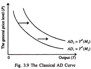
Since the quantity theory of money is an implicit theory of the aggregate demand for output in the classical model, we can use this to construct the classical aggregate demand curve, as shown in Fig 3.9. The classical aggregate demand curve (AD,) is a locus of points showing combinations of P and Y consistent with the quantity theory equation PY = M, for a given money supply (M) and fixed velocity (V).

An in­crease in money supply from M₁ to M₂, ceteris paribus, shifts the aggregate de­mand curve to the right — from AD₁ to AD₂.

Price and Output Determination in the Classical Model:

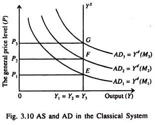
For a given quantity of money, there is one downward sloping aggregate demand curve. This, together with the vertical AS curve in Fig. 3.10 determines both P and Y in the classical model. Every time money supply increases the AD curve shifts to the right, from AD₁ to AD₂ to AD₃.

As a result the price level rises from P₁ to P₂ to P₃. But output which is supply determined remains unchanged (Y₁, = Y₂ = Y₃). Moreover, since k (or V) remains con­stant, a change in M is the only factor that shifts the aggregate demand curve.

The classical theory does not focus on the components of aggregate demand and so it does not explain the factors that determine their level. Instead, in the classical theory,
a given value of MV [or M (1/V)] implies the level of P x Y that is required to ensure money market equilibrium: M = M^d. If demand for money exceeds (falls short of) supply of money, people will try to reduce (increase) their expenditures on commodities.

Points along any aggregate demand curve are points at which firms and households are in equilibrium with regard to their money holdings and, therefore, are also at equilibrium rates of expenditures on commodities.