Agricultural Stabilization Schemes and Its Problems

In this article we will discuss about the agricultural stabilization scheme and its problems.

In free-market economies, farm incomes often tend to fluctuate around a low average level.

Agricultural-stabilization programmes have two goals:

(i) To reduce the fluctuations and

(ii) To raise the level of farm incomes.

Most countries now operate some sort of scheme to reduce agricultural fluctuations. The two policies, producing stable incomes and producing reasonably high incomes, can often conflict. We shall illustrate the workings of agricultural stabilization schemes for unplanned fluctuations in supply. A similar analysis could be carried out for cyclical fluctuations in demand.

Figure 2 shows the demand and supply curves for some farm product. The supply curve shows planned production at each price and, if production could be planned with certainty, price would settle down at the equilibrium level of OP. Although planned production is at OM₁ actual production fluctu­ates around that level, say between the quantities OM, and OM₂. In a free market, price will thus fluctuate between OE and OF.

One method of preventing these fluctuations in prices and incomes is for individual farmers to form a farmer’s association which tries to even out the supply actually coming on to the market, in spite of variations in output.

“There is no point in an individual farmer holding some of his production off the market in an effort to force up the price. Since one farmer’s production is a completely insignificant part of total production, the farmer who sold less would only reduce his income without having any noticeable effect on price. But if all farmers get together and agree to vary the supply coming on to the market, then, collectively, they can have a major effect on prices.”

Under the conditions illustrated by Figure 2, a farmer’s association might succeed in keeping the prices at OP and incomes at the level indicated by the area of the rectangle OPAM. Any excess of production over OM would have to be stored away unsold. If, production for one year were OM₂ then MM₂ would have to be added to the association’s stocks while OM was sold at the price OP.

Any deficiency of production below OM on the other hand, would have to be made good by sales out of the association’s stocks. If production were OM₁, for example, then M₁M would be sold out of stocks, making total sales again equal to OM at a price of OP.

In this way the farmer’s association could keep sales, price and incomes stabilized in spite of fluctuations in output. Provided the level of sales to be maintained (OM in our Figure 2) were equal to average production, theft, the policy would be carried on indefinitely: If on the other hand, an attempt were made to keep the price too high, so that sales were less than the average production then, over a number of years, additions to stocks would exceed sales from stocks, and the level of stocks held would tend to increase.

The successful policy is the one that keeps sales constant at OM (by adding to, or subtracting from stocks) and, since income accrues to the producers when the products are actually sold on the market, incomes will be stabilized at OPAM.

What will happen if a farmer’s association is not formed but the Govt., attempts to stabilize the incomes of farmers by entering the market itself, buying in the open market and adding to its own stocks when there is a surplus, and selling in the open market, thus reducing its stocks, when there is a shortage? If the Govt., wishes to stabilize farmers incomes, what policy should it adopt? Should it aim, at keeping prices constant at all times?

If the average level of production around which the year-to-year figure fluctuates is OM then there, is no reason why the govt., should not successfully stabilize the price at OP indefinitely. This policy would not have the result of stabilizing farmers’ incomes.

Farmers will now be faced with an indefinitely elastic demand at the price OP: whatever the total quantity produced, they will be able to sell it at the price OP; if the public will not buy all the produc­tion, then the govt., will purchase what is left over, If total production is OM₂, then OM will be brought by the public and MM₂, by the govt., to and to its own stocks. Total farm income in this case will be the amount indicated by the area of the rectangle OPCM₂ (the quantity OM₂ multiplied by the price OP).

If total production in another year is only OM₁ then this quantity will be sold by farmers and the government also will sell M₁M out of its stocks so that price will remain at OP. Total farm income will then be the amount indicated by the rectangle OPBM₁, (quantity OM₁ multiplied by the price OP).

It is obvious that if prices are held constant and farmers sell their whole production each year, then farmer’s incomes will fluctuate in proportion to fluctuations in production. The government policy, therefore, will not eliminate income fluctuations but it will reverse their direction. Now bumper crops will be associated with high incomes while small crops will be associated with low incomes.

What, then, must the govt’s policy be if it wishes to stabilize farmers’ revenues through its own purchases and sales in the open markets? Too much price stability causes revenues to vary directly with production, as in the case just considered, while too little price stability causes them to vary inversely with production as in the free-market case originally considered. It appears that the govt. should aim at some intermediate degree of price stability. In fact, if it allows prices to vary exactly in proportion to variations in production, then revenues will be stabilized.

The govt. policy necessary to achieve the requisite price fluctuations is shown in Figure 3. As before, planned production is OM₁, and the price which equates demand with planned production is OP. Actual production, however, fluctuates between OM₁ and OM₂ and these fluctuations, given the very in­elastic demand’ curve DDQ, could cause price to fluctuate between OR and OQ.

Now construct through the point A (the equilibrium point when actual production is equal to planned production) a curve of unit elasticity through­out its whole, range. This constructed curve is the dotted rectangular hyper­bola in Figure 3, labelled η= 1. If OM is produced and sold at price OP, total income is that indicated by the rectangular OPAM. The dotted curve now tells the market price that must rule if production and sales are allowed to vary but income is to be held constant at OPAM.

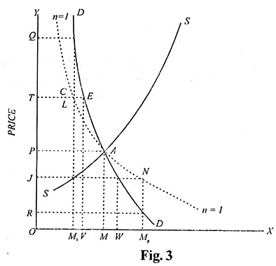
Consider first what happens if production is OM₂. Market price must be held at OJ (=M₂N) if income is to be unchanged. But, at market price OJ, the public only wishes to purchase OW (=JK) and it is therefore necessary for the government to buy up the remaining production. MW (=KN) and add it to its stocks. Farmer’s total sales are OM₂ at price OJ, and since the dotted curve is a rectangular hyperbola, it follows that income OJNM₂ is equal to income OPAM.

Now consider what must happen if production is equal to OM If farm income is to be unaltered, then the price must be allowed to rise to OT (by construction the area of rectangle OJLM₁ is equal to the area of rectangle OPAM). But at the price OT₁ the public will wish to buy OV (=TE) so that the government must sell LE out of its stocks.

If this policy is successful, it will have the following results:

(i) There will be smaller fluctuations in the price of this product than there would be if price were determined on a completely free market,

(ii) Total revenues of the producers will be stabilized in the face of fluctuations in production,

(iii) The government scheme should be self-financing.

In fact, if we ignore costs of storage, the scheme will show a profit, for the government will be buying at low prices (below OP)— the lower the price the more it buys—and it will be selling at high prices (above OP)—the higher the price the more it sells.

Whether or not the scheme actually shows a profit will depend on the costs of storing the crops from the periods of glut when they are purchased until the periods of shortage when they are sold.

In any case, this scheme has the financial advantage over the previous one in which the government completely stabilized prices, because in that case there would necessarily be a loss: since all purchases and sales would be made at the same price, OP There would be no trading profit to set against the costs of storage.

Problems with Agricultural Stabilization Policies:

One of the major problems with these agricultural stabilization schemes arises from the absence of perfect knowledge, combined with political pressure applied by farmers. Demand and supply curves are never known exactly, so the central govt. does not know what will be the average production forthcoming over a number of years at various prices. The central govt. does not know exactly what level of income it can try to attain while also keeping sales from stocks approximately equal to purchases for stocks, over a large number of years.

Since farmers have votes there is strong pressure on any govt. to err in the direction of fixing the income to be stabilized at too high a level. If the level of income and hence price, is fixed too high, then the central govt. will find it necessary to purchase unsold crops most of the years and will find only a few years when output is low enough for sales to be made out of stocks In this case, stocks will build up more or less continuously, and the time will come when no more can be stored.

When this happens, the stored crops will either have to be destroyed, given away or dumped on the market for what they will bring, thus forcing the market price down to a very low level. If the crops are thrown on the market and allowed to depress the price, then the original purpose for which the crops were purchased, price stabilization, is defeated.

If the crops are destroyed or allowed to decay, then this means that the efforts of a large quantity of the country’s scarce factors have been completely wasted. Furthermore, the govt’s plan will now show a deficit, for goods will have been brought which cannot be sold at all. This deficit will have to be made up by taxation which means that people in cities will be paying farmers for producing goods which are never consumed

When schemes get into this sort of difficulty, the next step is often to try to limit the production of each farmer. Quotas may be assigned to individual farmers and penalties levied for exceeding them.

Or else, bonuses may be paid for leaving land idle, for ploughing crops under without harvesting them, or for other means of cutting back on production. Such measures attempt to get around the problem that too many resources are allocated to the agricultural sector by the device of preventing these resources from producing all that they are capable of producing.

Resources in Agriculture: The Long-term Problem:

Even if the temptation to set too high a price is avoided, there is still a great problem waiting wreck many agricultural-stabilization programmes. This problem results from the fact that the productive capacity of almost all economies is growing over time. In U.K., the increase in per capita production has averaged almost 2% a year over the last 100 years.

Owing to better health, better working conditions, and more and better capital equipment, workers in most sectors of the economy can produce more per head than they previously did. If the allocation of resources were to remain unaltered there would be an increase in proportion to the increase in productivity in that industry.