Expansionary Fiscal Policy and Monetary Policy under Fixed Exchange Rate

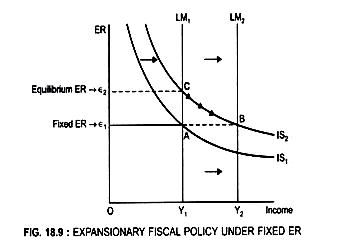
Initially, the economy is in equilibrium at point A.

At point A : IS₁ = LM₁

Fixed ER → є₁

If there is an Expansionary fiscal policy, it will lead to an increase in AD.

Result:

IS curve will shift to the right from IS₁ to IS₂ (Fig. 18.9)

At the given ER → є₁

Product market is in equilibrium at point B

But at point B, IS₂ ≠ LM₁

For both markets to be in equilibrium, ER has to rise from є₁ to є₂

Equilibrium will be attained at point C as here IS₂ = LM₁

But a point C: Equilibrium ER (є₂) > Fixed ER (є₁)

To maintain Fixed ER, Central Bank will buy $, (that is, the arbitrageur will sell $) to the Central Bank

Result:

Money supply of rupee will increase and LM curve will shift to the right from LM₁ to LM₂ till equilibrium ER is established at fixed ER (є₁)

Due to shift in LM curve, ER falls from є₂ to є₁ and Fixed ER becomes equal to the Equilibrium ER

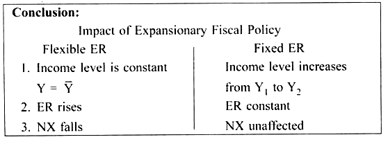
However, Income level will increase from Y₁ to Y₂.

Equilibrium will be at higher income level (Y₂)

This is at point B where IS₂ = LM₂ at higher income level → OY₂ but at same ER → є₁

Expansionary Monetary Policy Under Fixed ER With Price Level Fixed:

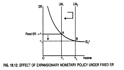
If Central Bank buys bonds from the public, money supply will increase.

Result:

LM curve will shift to the right from LM₁ to LM₂ as a result ER falls from є₁ to є₂ (Fig 18.12).

Fixed ER (є₁) > Equilibrium ER (є₂)

The arbitrageur will sell domestic currency (Rs) to the Central Bank and buy $

Result:

Money supply will decrease, and thus LM curve will shift back to the left from LM₂ to LM₁ (to its initial position).

ER will rise to є₁ and fixed ER will be maintained.