Consumer Equilibrium Formula | Microeconomics

In this article we will discuss about the consumer equilibrium formula with the help of suitable examples. 

Suppose, the utility function of the consumer is:

U = f (q₁, q₂)                                        [eq. (6.1)]

Where U is the ordinal utility number, and q₁ and q₂ are quantities of the two goods, Q₁ and Q₂, that the consumer purchases. It is assumed here that the first-order and second-order partial derivatives of U w.r.t. q₁ and q₂ exist.

Also suppose, the budget constraint of the consumer is given to be:

y^o= p₁q₁ + p₂q₂                                      (6.23)

where y^o is the fixed amount of income that the consumer spends on the goods Q₁ and Q₂, and p₁ and p₂ are the given prices of the two goods. It is intend to derive here the conditions for the utility-maximising equilibrium of the consumer subject to his budget constraint.

For that purpose, the following Lagrange function can be formed:

V = f(q₁, q₂) + λ(y^o – p1q1 – p₂q₂)     (6.24)

where λ is the undetermined Lagrange multiplier.

First-Order Condition for Utility-Maximisation:

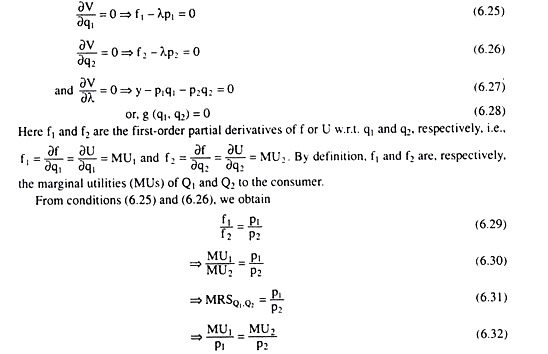
In (6.24) V is a function of q₁, q₂ and λ and the first order conditions (FOCs) of constrained utility-maximisation would be obtained if the first-order partial derivatives of V w.r.t. q₁,q₂ and λ equal to zero.

Therefore, these FOCs are:

 

 

 

 

 

 

 

 

 

 

 

 

 

 

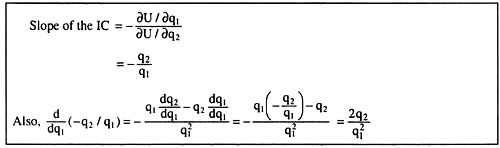
Equations (6.29) − (6.32) gives the different forms of the FOC for constrained utility-maximisation. The left-hand sides (LHSs) of (6.29) − (6.31) gives the numerical slope of the indifference curve (IC) and the right-hand sides (RHSs) gives the ratio of the prices of the two goods, or, the numerical slope of the budget line.

Therefore, the FOCs as given by (6.29)-(6.32) all gives the first-order or the necessary condition for utility maximisation would be satisfied at the point of tangency between the budget line and an IC of the consumer.

The FOC for utility-maximisation as given by equation (6.32) states that utility will be maximised if the consumer spends his money on the two goods in such a way that the rate of change of utility or satisfaction w.r.t. money spent on each good may become the same.

If he divides the spending of money between the two goods in such a way that the rate of change of satisfaction w.r.t. money spent on one good is more than that on the other good, then the con­sumer would not be able to maximise the level of utility by spending all his money on the two goods.

Now, he would have to spend more on the former good and less on the latter till the rate of change of satisfaction from the former good decreases and that from the latter good in­creases for the two to become the same.

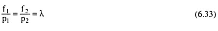
Lastly, from the first-order equilibrium conditions (6.25) and (6.26), it is obtained that:

when MU of money spent on each good becomes the same, it amounts to the MU of income. Therefore, (6.33) gives the Lagrange multiplier A, can be interpreted as the marginal utility of income.

Since the MUs of the commodities are assumed to be positive (for the goods are assumed to be MIBs), the MU of income is also positive. Also note that equation (6.27) of the FOC ensures that the budget constraint has been satisfied.

Second-Order Condition:

Now come to the second-order condition (SOC) or sufficient condition of utility maximisation.

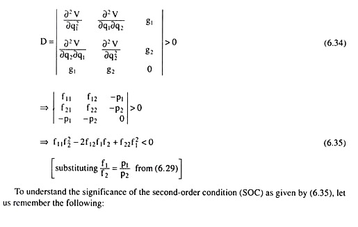
The SOC states that the bordered Hessian determinant, D, should be greater than zero at the point of tangency where the FOC has been satisfied:

 

 

 

 

 

 

 

 

 

 

 

 

 

 

 

 

 

 

 

 

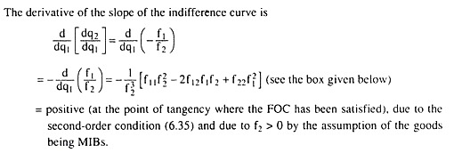
Therefore, the SOC implies that the derivative of the slope of the IC would be positive, i.e., the IC would be convex to the origin at the point of tangency. Since any point on an IC may be the point of tangency depending upon the slope of the budget line, the SOC actually implies that the IC should be convex to the origin throughout its length.

It may be noted here that, since the second-order or the sufficient condition (6.35) for consumer equilibrium is satisfied at each point within the domain of a regular strictly quasi-concave function, the utility function (6.1) of the consumer should be a regular strictly quasi-concave function. Only then the second-order condition would be satisfied.

Example:

Assume that the utility function is U = q,q₂, and p, = 2 (Rs) and p₂ = 5 (Rs), and the consumer’s income for the period is y = 100 (Rs). Find the commodity combination that would maximise the consumer’s level of satisfaction subject to his budget. Also, find the marginal utility of income at the equilibrium point,

Solution:

The utility function has been given as

U = q₁q₂ (i)

 

 

 

 

 

 

 

 

 

 

 

 

 

 

 

 

 

 

Therefore, it is obtained from the FOCs that the utility-maximising quantities of the goods are q₁ = 25 units and q₂ = 10 units.

Now verify whether these quantities satisfy the second-order condition (SOC) for utility-maximisation. This condition is

 

 

 

 

 

 

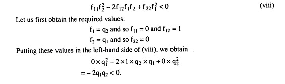
Therefore, the SOC as given by (viii) is verified. So, finally, the equilibrium quantities are q₁ = 25 units and q₂ = 10 units, and the MU of income is already obtained to be λ = 5 which is an ordinal utility number.

The example can be presented graphically with the help of Figure 6.11. The ICs in the given example are rectangular hyperbolas, as is evident from the utility function (i). Two such ICs, viz., IC₁ and IC₂, have been given in Figure 6.11.

The budget line as given by equation (ii) is the line LM. It is obtained from (ii) that the q₁-intercept of the budget line is 50 units and the q₂-intercept of the budget line is 20 units.

That is, if the consumer spends all his money (100) on Q₁ at p, = 2, he would be able to buy 50 units of Q₂ and if he spends all his money on Q₂ at p₂ = 5, he would be able to buy 20 units of Q₂. The numerical slope of the budget line or the price ratio is p₁/p₂ = 2/5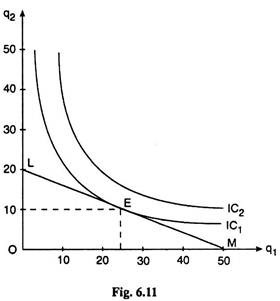

The FOC for consumer equilibrium has been satisfied at the point of tendency E. At this point the MRS_Q1,Q2 =  (∂U/∂q₁)/(∂U/∂q₂) = q₂/q₁ = 10/25 = 2/5 has been equal to the price ratio p₁/p₂ = 2/5. As regards the SOC, the derivative of the slope of the IC w.r.t. q₁ at the point E = d/dq₁ (-q₂/q₁) = + 2q₂/q₁ = positive, i.e., the IC is convex to the origin at the point E, and the SOC is satisfied.