Samuelson Model and Super-Multiplier Model of Business Cycle

Read this article to learn about the concept, importance and limitations of the Samuelson and Super-Multiplier model of business cycle.

Concept of the Models:

Consumption and investment spending as determined by a certain set of relationship interact with each other to form the propelling force for aggregate change, which in turn, forms the basic explanatory variable for further changes in both consumption and investment.

This accelerator-multiplier model must be considered as a first approximation for the understanding of the basic forces that determine the behaviour of the economy. In other words, the determinants for our spending streams are more complicated than those given by the assumption of the model.

The assumptions are:

(a) That consumption spending in the current period is related to income in the preceding period;

(b) That investment in the current period is related to the change in income with a lag of one period;

(c) There is also an additional factor in the form of exogenous (government) spending, which is a constant equal to;

(d) The model does not consider the determinants of this exogenous spending nor the effects of its changes on the level of income.

Thus, the true structure of the model stems from the nature of lags and the coefficients α and β which relate the variables in the equation. Assuming the one—period lag as a given tolerable approximation of economic behaviour; we next set out the values of our coefficients that results in changes in the level of Y. We discern mainly five types of changes as discussed further.

Thus, Paul Samuelson studies the interaction of the multiplier and accelerator in greater details and derived a model in which a series of equations express the way in which the two forces interact to affect income, consumption and investment over a time. The accelerator investment function so far used has been — I_t– I_a + w (Y_t – Y _t-1).

This function is but one of a group of possible investment functions incorporating the acceleration principle. Instead of making the accelerator apply to the change in total output, Y_t – Y _t-1 another function in this group makes the accelerator apply only to the change in the output of consumer goods, C _t– C _t-1. Hence, the resulting function is: I_t + I_a w(Ct – C_t–₁). This is the function used in Samuelson’s model. Still other functions result from employing a lagged acceleration instead of the un-lagged as used above.

As such, I_t– l_p + w (Y_t-1– Y_t– ₂) or if we use lagged consumption instead of lagged income, we have, I_t= I_a + w (C _t-1 – C _t-2), The lagged function is more realistic because lagged functions allow for an interval of time between the decision to invest and the actual investment.

Similarly, in the case of consumption function, we may work with lagged or un-lagged relationships. The earlier CF is un-lagged (C_t = C_a + cY_t), it assumes that the consumption of each period depends on that period’s autonomous C and on that period’s Y. The alternative of this un-lagged CF is the lagged CF (C_t= C_a + cY_t–₁): it assumes that consumption in each period depends on that period’s autonomous consumption and the preceding period’s income.

Since Y_t = C_t + I_t..By substituting the values of C₁ and I_t as shown above, we get:

Y_t= C_a + cY _t-1 + l_a + W (C_t – C_t–₁).

This equation shows that aggregate income or output in a period (Y_t) equals the sum of autonomous consumption (C_a) and autonomous investment (I_a) plus an additional amount of consumption that depends upon the mpc (c) times the income of the preceding period (Y _t-1); and an additional amount of investment that depends on the capital-output ratio or the accelerator (w) times the change in consumption between the current and the preceding period (C_t – C _t-1). In other words, if we know C_a and I_a for any period and C for the current and preceding periods, we can, given the values of c and w, determine the growth path of income and output of any period by substituting in the equation for Y, given above.

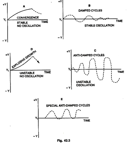
In his paper, Samuelson set forth the various patterns of change that the level of income might display for different combinations of values of c and w, given a change in autonomous spending that upsets a previous equilibrium. This is shown in four cases or five if we include a special case given in Fig. 42.2.

In Fig. 42.2(A), income moves upward or downward at a decreasing rate and approaches a new equilibrium, in (B), income fluctuates through a series of cycles of smaller and smaller amplitude until the cycles virtually disappear; in (C), income fluctuates through a series of cycles of wider amplitude; in (D) income moves upward or downward at an increasing rate. In (E), (which is a special case) income fluctuates through a series of cycles of constant amplitude.

We have seen that multiplier and accelerator working together give us the process of income generation. But Professor P.A. Samuelson went further and showed that with different combinations of the values of the multiplier and accelerator, it is possible to get income fluctuations (cycles) of various types, as shown in Fig. 42.2.

In a much-quoted article Interaction Between the Multiplier Analysis and the Principle of Acceleration Reprinted in Readings in Business Cycle Theory, 1944, he showed that with different values of the Marginal Propensity to Consume (c) on the one hand and the Acceleration (w) on the other, it is possible from a continued injection of public different types of cycles or fluctuations. If we express MPC as a (Alpha) and acceleration coefficient as 3 (Beta), the five types of cyclical fluctuations are already shown on below.

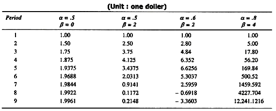
The table given from Samuelson is more illustrative:

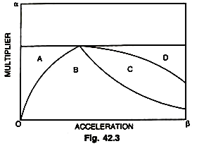
1. α = 0.5 and β = 0—This gives us purely multiplier effects with income approaching the peak. Here the acceleration coefficient is zero (Region A in the diagram 42.3). This is the case of fluctuations having multiplier effect only; where income approaches asymptotic level.

The system will not exhibit any fluctuations. If the economy experiences a single impulse of expenditure and then a complete stop income will initially increase by the amount of the impulse but will thereafter begin to decrease. Subsequent income levels, being determined by consumption expenditures only, will result in negative income changes as mpc < 1.

2. α = 0.5, β = 1—This gives us damped oscillations, falling in value as they fluctuate about that multiplier level, gradually subsiding to that level. (Region B in the diagram 42.3). The system will kick up only to slide to a cyclical path and will approach the new static position of the multiplied level of the constant expenditure.

3. α = 0.5, β = 2—This gives us regular or continuous cycles about the multiplier level with more or less unchanged values repeating themselves indefinitely.

4. α= 0.6, β = 2—This gives us explosive cycles with variations about the multiplier level becoming large and large. (Region C in the diagram 42.3).

5. α = 0.8, β = 4—This gives us an ever increasing income gradually approaching a compound interest rate of growth (Region D in the diagram 42.3).

These five cases show self-generating or endogenously determined patterns of change resulting from the interplay of consumption and investment determinants. We see that only cases 2 to 5 give rise to cyclical patterns, which, of course, reflects the behaviour of the real economy.

Generally, the cycles in the post-war period have been relatively damped compared to those in the inter-war period. But the dampening has been irregular and our observations are too few and methods so inadequate that they don’t provide any definite conclusions about the amplitude of future cycles, much less to predict whether they will continue to exist. However, there is no evidence to support the view that cycles will completely die out.

Certain timely fiscal, monetary and other measures may restrict the amplitude of the cycles but the dampening factors will continue to operate as a result of the changing character of the private forces that flow or originate from within the economy itself. This leaves us with explosive cycles of the type mentioned in cases 4 and 5. However, if cycles have not been dying out, there is no reason to presume that they behaved in the past or will behave in future in an explosive manner.

We summaries the below results. In this diagram, region A shows the first case of multiplier effects only where the value of p (accelerator) is zero. In this case, with a constant level of public expenditure, the national income will reach its peak by multiplier value only (i.e., 1/1-α times or 1/1-[1/2]=2)

Region B shows damped oscillations in value as they fluctuate about the multiplier level. Region C shows explosive cycles with variations about the multiplier level becoming larger and larger and region D shows the ever increasing national income approaching a compound interest rate of growth.

The essence of the argument is that multiplier- accelerator interaction is capable of generating various types of cycles and fluctuations: mild, damped and explosive. These cycles or fluctuations are of varying periodicity and magnitude depending on the values of c and w. Professor J.R. Hicks has used this mechanism in building up a theory of the trade cycle that explains the behaviour of business cycle during the rising trend of income.

The various types of movements that result from the multiplier- accelerator interaction have provided the basis for two groups of business cycle theories. In one group are included the theories of economists like Hicks and Goodwin, who have built theories on the assumption that the values of c and w are such as to produce anti-damped or explosive cycles. Hansen is the chief name in the other group, who is the leading advocate of weak accelerator theory. In his view, the interaction produces only damped cycles. The general opinion appears to support the anti- damped cycle.

Importance:

Thus, we find that Super-Multiplier (interaction of multiplier and accelerator) assumes greater importance inasmuch as it appears to speed up the rate at which the national income rises than by the multiplier effects. The study of the interaction of the two principles has paved the way for a more accurate analysis of the nature of the cyclical processes, further, an analysis of the interaction shows that it is possible to explain turning points in business cycles without resorting to special explanation. These factors are: a marginal propensity to consume of less than one plus the acceleration effect, the former being perhaps more important.

The acceleration principle, before Keynes, was based on Say’s Law, wherein increase in the rate of consumption gives rise to a proportionate increase in investment and a decrease in the rate of consumption would lead to a similar decline in investment—i.e., a cumulative expansion or contraction without limit. Thus, the pre-Keynesian theory of acceleration principle gave an exaggerated picture of the instability in the economy.

But with the introduction of the concept of multiplier and consumption function of less than unity, the long-sought for limits to the fluctuations short of zero were at last found. Keynesian concept of consumption function has brought forward the true significance of the acceleration principle for business cycle analysis.

According to Prof. K. Kurihara, “It is in conjunction with the multiplier analysis based on the concept of the marginal propensity to consume (being less than one) that the acceleration principle serves as a useful too for business cycle analysis and as a helpful guide to business cycle policy.” The combination of the multiplier and the accelerator seems capable of producing ‘cyclical fluctuations.’

The multiplier alone produces no cycles from any given impulse but only a gradual increase to a constant level of income determined by the propensity to consume. But if the principle of acceleration is introduced, the result is a series of oscillations about what might be called the multiplier level. The accelerator at first carries total income above this level, but, as the rate of increase of income diminishes, the accelerator induces a downturn which carries total income below the multiplier level, than up again, and so on.

Limitations:

A casual student of super-multiplier (multiplier-acceleration principle) might feel that it is very easy to raise the economy out of the depths of depression simply by having a small increase in autonomous investment. This would stimulate consumption via the multiplier effects, which would then induce further investment and the national income would continue to grow like a Topsy. Such a possibility is a great illusion.

In actual practice, the interaction of the multiplier and acceleration does not go to raise the national income to higher and higher levels; at best, it is responsible for fluctuations on the path of movement of national income from one level to another. The interaction, no doubt, shows significant cyclical effects but there are many practical difficulties in the actual calculations of the total effects of the multiplier and acceleration principle.