Theory of Distribution: Top 44 Things to Know About

The following points will highlight the top forty four things to know about the theory of distribution. The things are: 1. Subject-Matter of the Theory of Distribution 2. Rent 3. Rent of Land 4. Economic Rent and Transfer Earnings 5. Interest 6. Interest and Credit 7. Length of Loan 8. Risk 9. Administrative Charges 10. Interest Rate in Future and Present Values and other things.

Theory of Distribution # 1. Subject-Matter of the Theory of Distribution:

Much of our material will be familiar because the same factors that shape the demand and supply in output markets also affect factor markets. Factor markets, like output markets, can differ greatly in their structure.

We will examine three different factor market structures:

(1) Perfectly competitive factor markets,

(2) Markets where buyers of factors have monopsony power, and

(3) Markets where sellers have monopoly power. We will also discuss equilibrium in the factor market.

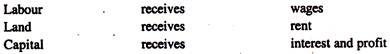
This involves the study of the functional distribution of income.

There are three major divisions of income which the factors of production receive:

According to traditional distribution theory, the distribution of income is simply a special case of price theory.

This can be summarised in three major points:

(1) The income of any factor of production (and, hence, the amount of the national product that it is able to command) depends on the price that is paid for the factor and the amount that is used.

(2) Factor prices and quantities are determined by demands and supplies in factor markets in exactly the same way that prices and quantities of commodities are determined in commodity markets.

(3) To explain distribution of income through price theory it is necessary to identify the main determinants of demand for — and supply of — factors of production. It is also necessary to allow for any intervention into free markets caused by governments, trade unions or other similar institutions.

Fig. 14.1 illustrates the concept of economic rent as applied to the competitive labour market. The equilibrium price of labour is W_e, and the quantity of labour supplied is L_e. The supply of labour curve is the upward- sloping average expenditure curve, and the demand for labour is the downward- sloping marginal revenue product curve.

Since the supply curve of labour tells us how much labour will be supplied at each wage rate, the minimum expenditure needed to employ L_e units of labour is given by the area AL_e OB, the area below the supply curve to the left of the equilibrium labour supply L_e.

In perfectly competitive markets, all workers are paid the wage W_e. This wage is required to get the marginal workers to supply their labour, but all other infra-marginal workers earn rents because their wages are greater than what would be needed to get them to work.

Since total wage payments are equal to the area OW_e AL_e, the economic rent earned by the worker is given by the area ABW_e. From the worker’s point of view, economic rent is similar to consumer’s surplus.

Theory of Distribution # 2. Rent:

Now we discuss rent of land. We define economic rent in output markets as the payments received by a firm over and above the minimum cost of producing its output. For a factor market, rent is the difference between the payments made to a factor of production and the minimum amount that must be paid to obtain the use of that factor. Note that if the supply is perfectly elastic, economic rent would be zero.

Rents arise only when supply is inelastic. If the supply is perfectly inelastic, all payments to a factor of production are economic rents because the factor will be supplied no matter what price is paid. The best example of in elastically supplied factor is land, as in Fig. 14.2.

Theory of Distribution # 3. Rent of Land:

Rent arises from the inelasticity of supply, when the supply is perfectly elastic, economic rent would be zero. The supply of land is inelastic. Thus, the supply curve for land is a vertical line as in Fig. 14.2. That is to say, no matter what the prevailing market price for land, the quantity supplied will remain the same. The term “rent” has been associated with payment for the use of land.

When the supply of land is perfectly inelastic, Rent the price of land is determined at the point of intersection of the dc, and the entire value is economic rent. When demand is D, the economic rent per area is given by S₁ and when demand is increased to D₁ the rent increases to S₂.

When, indeed, no matter what the price, the quantity and quality of a resource will remain at its current levels, we say there is pure economic rent. We define pure economic rent as that price paid to land that is in completely inelastic supply. It is also a term used for any payment in excess of that needed to keep a particular factor in its current use.

This is different from common use of the term “rent” which includes a payment for the use of land as we pay wages for the use of labour.

Ricardo used rent as a payment for the “original and indestructible qualities of soil” on the assumption that land has only one use — that of growing foodstuff. Thus, he pointed out that the supply of land is fixed — its supply price is zero. It is the community’s demand for foodstuff that determines the demand for land. In other words, the demand for land is a derived demand.

Fig. 14.2 shows the perfect inelasticity of the supply of land, SS, intersecting the community’s demand for land, DD. The equilibrium rent is OR. Now, suppose, the demand for land increases to D₁D1. This will raise the equilibrium rent from OR to OR₁. Thus, the rent is demand- determined.

Theory of Distribution # 4. Economic Rent and Transfer Earnings:

Ricardo’s theory of rent assumes a fixed supply of land so that all rent is a surplus over and above the cost of keeping land in its present use. Such surplus has become known as economic rent and it has been pointed out that it can be expanded to other factors as well.

We now define economic rent and transfer earnings. Transfer earnings are the payment required to keep a factor in its presents use. Economic rent is any payment in excess of transfer earnings.

Theory of Distribution # 5. Interest:

Interest is the price paid for the use of capital. Capital is a man-made factor of production. Capital exists because individuals in the past have been willing to forgo consumption — to save. Those resources, not consumed, were usually used by firms for investment purposes, which added to the stock of capital.

The production of capital goods occurs because of the existence of credit markets, where borrowing and lending take place.

Owners of capital obtain income in the form of interest. They receive a specific interest rate. Thus, we can look at the interest rate as either the rate earned on capital invested or the cost of borrowing — two sides of the credit market. Here we will look only at the cost of borrowing.

Theory of Distribution # 6. Interest and Credit:

When we obtain credit, we actually obtain money to have command over resources today. Thus, the interest rate is the payment for current rather than future command over resources. Interest is the payment for obtaining credit.

The interest that we pay is usually expressed as a percentage of the total loan calculated on an annual basis. If, at the end of one year, we pay £110 for £100, the annual interest is 10%. We know that the interest rate charged differs greatly.

Variations in the rate of interest depend on the following factors:

Theory of Distribution # 7. Length of Loan:

In some cases, the longer the loan will be outstanding, other things being equal, the greater will be the interest rate charged.

Theory of Distribution # 8. Risk:

Greater the risk of non-payment of the loan, other things being equal, greater is the interest rate charged. Risk is assessed on the basis of credit-worthiness of the borrower. It is also assessed on the basis of whether the borrower provides collateral for the loan.

Collateral consists of any asset that will automatically become the property of the lender should the borrower fail to comply with the loan agreement. The more and better the collateral offered for a loan, the lower the rate of interest charged, other things being equal.

Theory of Distribution # 9. Administrative Charges:

It takes resources to set up a loan. Papers have to be filled and filed, credit references to be checked, and so on. It turns out that the larger the amount of the loan, the smaller will be the administrative charges as a percentage of the total loan. Therefore, we would predict that, ceteris paribus, the larger the loan, the lower the interest.

Loans are taken out by both consumers and firms. We will treat consumption loans and investment loans, separately. Before we do that, we examine the relationship between interest rates and present value — or how to relate the value of future sums of money to the present. In the discussion that follows, it will be assumed that there is no inflation.

Theory of Distribution # 10. Interest Rate in Future and Present Values:

Interest rates are used to link the present with the future. After all, if we have to pay £110 at the end of the year when we borrow £100, that 10% interest rate gives us a measure of the price of things, one year from now, compared to the price of things today. If we want to have things today, we are to pay the 10% interest rate in order to have purchasing power.

The question could be asked this way: What is the present value of £110 that we receive one year from now? That depends on the market rate of interest, or the rate of interest we could earn in a bank account. Let us assume that the rate of interest is 10% (called rate of discount). Now we can find out the present value of £110, to be received next year.

We can find out by answering the question: How much money must we put aside today at a market rate of interest of 10% to receive £110 one year from now?

Mathematically:

(1+ 0.1)P = £110, where P is the amount of money to be set aside now:

P==£100

That is, £100 will accumulate to £110 at the end of one year with a market rate of interest of 10%. The formula for the present value of any sums to be received one year from now is:

P=

where P = present value, A = future sum of money received one year hence, r = market rate of interest.

The same method can be used to calculate the present value of income expected in the more distant future. This discounting helps firms to assess the present value of the income they are likely to receive from an investment project.

Theory of Distribution # 11. Determinants of Interest Rates:

The neo-classical theory tells us that the level of interest rate in the economy is determined by the demand and supply of loanable funds. Let us look at the supply side first.

Theory of Distribution # 12. Supply of Credit or Loanable Funds:

The supply of loanable funds depends upon interest rate. Thus, the supply curve of loanable funds will be upward-sloping, as in Fig. 14.3. At higher interest rates, savers will be willing to reduce current consumption, other things being equal.

Theory of Distribution # 13. Demand for Loanable Funds:

The demand for loanable funds is the sum of individual firm’s demand, consumers demand and the government’s demand.

Theory of Distribution# 14. Firms’ Demand for Loanable Funds:

Firms demand loanable funds to make investments. If a firm believes that, by making an investment in its production process, it can increase revenues by more than the cost of capital, it will borrow and invest. Firms compare the interest rate that they are required to pay in the loanable fund market with the rate of return or profit they think they can earn by investing.

If the rate of return is greater than the rate of interest, they will invest.

At higher rates, fewer investment projects make economic sense — the cost of capital will exceed the rate of return on the capital invested. Conversely, at lower interest rates, more investment projects will be undertaken because the cost of capital will be less than the expected rate of return on capital invested, called marginal efficiency of capital.

Theory of Distribution # 15. Consumer Demand for Loanable Funds:

The demand by consumers for loanable funds will be inversely related to the cost of borrowing — the rate of interest. For the same reason that all demand curves slope down a higher rate of interest means a higher cost of borrowing, and a higher cost of borrowing must be weighed against alternative uses of limited income. At higher cost of borrowing, the consumer will forgo current consumption.

The demand for loanable funds comes from consumers (households), firms and the government, and the supply of loanable funds interacts to produce an equilibrium interest rate as shown in Fig. 14.4.

The funds are traded on the capital or money markets. This is one market which will clear all the time. Interest rates are flexible and the financial institutions can lend to one another on a short-term basis should there be excess supply of — or demand for— funds.

Theory of Distribution # 16. Real versus Nominal Interest Rates:

Until now, we have assumed that there is no inflation. In a world of inflation, nominal interest rates will be higher than they would be in a world with no inflation. Basically, market rates of interest rise to take account of anticipated rate of inflation.

If there is no inflation and no inflation expected, the market rate of interest might be 5%. If the rate of inflation goes to 10% a year, then everybody will anticipate that inflation rate will be higher.

The market or nominal rate of interest will rise to 15% to take account of the anticipated rate of inflation. Thus, the real rate of interest is equal to nominal rate of inflation minus the rate of inflation. We can expect to see high nominal rate of interest in periods of high and rising inflation. Real rate of interest, though, may not necessarily be high.

Theory of Distribution # 17. Allocative Role of Interest:

The interest rate is the price that allocates funds to consumers and to firms. Within the business sector, interest allocates funds to different firms and to different investment projects. Those investment projects whose rate of return are higher than the market rate of interest will be undertaken, given an unrestricted market for loanable funds.

It is important to remember that the interest rate performs the function of allocating capital but what that ultimately does is it allocates real physical capital to various investment projects.

Theory of Distribution # 18. Profits:

Profit is the reward for entrepreneurial talent which is the fourth factor of production. Entrepreneurship involves engagement in the risk of starting new business. In a sense, nothing can be produced without an input of entrepreneurial skills.

Theory of Distribution # 19. Is Economic Profit a Payment for Managerial Skill?

Profit is not a reward for good management, because managerial skill is a service available in the market. Any entrepreneur can hire a manager. Better managers earn higher salaries than poor ones. The good entrepreneur who earns apparently high profits because of his good management is only earning an imputed salary — what he would have earned elsewhere by managing someone else’s business.

Strictly speaking, economic profit cannot be called the reward for managerial skill. Unlike a manager who might be employed by the owner, the person owning the enterprise takes the risk. It is, therefore, often argued that profits are the reward for taking such risks. After all, if the business fails, it is the owner who suffers a reduction in net worth. However, many risks can be reduced by purchasing insurance policies.

Theory of Distribution # 20. What is Profit?

Profit is residual. But it does not arise accidentally; it is a result of the unique capabilities of the firm’s owner. It is the reward of taking risk which cannot be covered by insurance. It can be explained in other ways too.

Theory of Distribution # 21. Exploitation:

The classical economists’ view of profit was indistinguishable from what we would now call interest. This is because their concern was not for individual market and individual factor prices, but rather for the share of national income earned by various social classes.

Karl Marx argued that the source of profits was exploitation. According to Marx, firms actually exploit workers by paying them less than what their labour was worth.

Marx based his argument upon the labour theory of value which stated that the force underlying the value of all goods was the amount of labour to produce them. This amount included “direct” labour — the actual amount used of labour of average skill — and “indirect” labour — the labour value of the portion of the tools used in producing the commodity.

Marx put forward his exploitation thesis by asking:

If the value of any commodity is measured by the direct and indirect labour-time needed to produce it, what can the value of labour-time itself be? He answered that it must be subsistence — the amount of goods and services needed to enable a worker and his family to keep body and soul together. This is the cost to the society to produce one worker. Thus, when the worker earned subsistence, he was earning a “fair wage.”

Marx was restating what all the classical economists believed:

Owners of firms earned profit because they could legitimately claim anything left over after all costs of production had been paid. Thus, according to Marx, the source of profit was exploitation — because the workers produce goods of much higher value than the price of their subsistence; by the rules of the game of capitalism itself, “exploitation” was a profit after perfectly fair.

Theory of Distribution # 22. Restrictions on Entry:

Monopoly profits are possible when there are barriers to entry. Monopoly profits due to entry restrictions are often called monopoly rents. Entry restrictions exist in many industries, such as taxis, prescription drugs, etc. Basically, monopoly profits are capitalized into the value of the business that owns the particular right to have the monopoly.

Theory of Distribution # 23. Innovation:

Economic profits are also created by innovation, which is defined as the creation of a new organizational strategy, new marketing strategy or a new product. The innovator creates new economic profit opportunities by innovations. The successful innovator obtains a temporary monopoly position, allowing him to have temporary economic profits.

Theory of Distribution # 24. Function of Economic Profit:

In a market economy, the expectation of profits induces firms to innovate. Profits, in this sense, spur innovation and investment. Profits cause resources to move from lower-valued to higher-valued uses. Prices and sales are dictated by the consumer. The lack of profits, therefore, means that there is insufficient demand to cover the opportunity cost of production.

Theory of Distribution # 25. Demand and Supply of Labour:

Here we will try to find out the amount of labour input that firms might demand and the price they are prepared to pay for them. We assume that labour is the only variable factor input and that all other inputs are fixed. A firm’s demand for labour can be studied in the same way as we studied the demand for products.

We assume that a firm will hire labour up to the point where it becomes unprofitable to hire any more, i.e., up to the point where the marginal benefit of hiring a worker just equals the marginal cost. We further assume that the market for labour is perfectly competitive, and that, the output market is also perfectly competitive. We will do away with these assumptions as we go along.

Theory of Distribution # 26. Competitive Product and Factor Markets:

A firm sells its product in a perfectly competitive market and also buys its labour input in a perfect market. The firm can influence neither the price of its product nor the price of labour input, but it can buy as much as it wants at a going market price. The going wage rate is fixed in the market by the forces of demand and supply. The total market demand for labour is the sum of all the individual firms’ demand for it.

Theory of Distribution # 27. Marginal Physical Product:

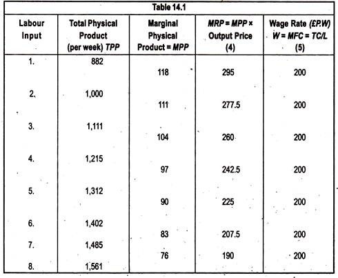
Table 14.1, Column 1, shows the number of workers-weeks that the firm can hire. Column 2 shows total physical product (TPP) that the different quantities of labour input can produce in a week.

Column 3 shows the additional output gained when a firm adds additional workers to its fixed capital; that means marginal physical product (MPP), which represents the extra output from the additional labour input employed. If the firm adds a second worker, the MPP is 118.

We know that the law of diminishing marginal returns will operate as more and more of variable factors are employed with the fixed amount of other factors.

Theory of Distribution # 28. Why does MPP Decline?

If more and more workers are added with the same capital stock, each worker has a smaller and smaller fraction of capital stock to work with. If one worker uses one machine, adding another worker will not normally double the output, because the machine can run only so many hours per day.

Theory of Distribution # 29. All Workers Paid Same Wage:

Since we have assumed competitive labour market, then every worker must be paid the same wage-rate. In Table 14.1, we assumed that the wage-rate is £200 per week. In addition, we need to know the price of the product. Since we have assumed perfect competition, the hypothetical market equilibrium price is £2.50, as in Table 14.1.

Firm will employ workers up to the point where MR = MC = Wage rate. The MC of workers is the extra cost we incur in employing that factor of production.

Theory of Distribution# 30. Marginal Revenue Product:

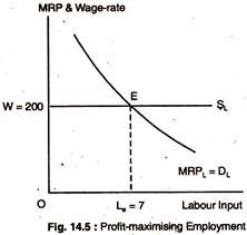
We now need to translate the MPP into MRP (money value). MRP = MPP x P of the product. If the second worker’s MPP is 118 and the market price of output is £2.5, then the MRP is £295 (118 x 2.50). We call the individual worker’s contribution to TR — the MRP. Fig. 14.5 shows the relationship between MRP = MC = wage rate, which gives profit-maximising firm’s employment generation.

In a perfectly competitive labour market, the wage-rate of £200 per week really represents the supply curve of labour.

Theory of Distribution # 31. How many Employees?

The firm hires workers up to the point where the MC is equal to the MR generated by that worker:

In a perfectly competitive market, this point is where the wage-rate = MRP. If the firm hires more workers, the additional wages would not be sufficiently covered by additional increases in total revenue. If the firm hires fewer workers, it would be forfeiting the contributions that those workers could make to total profits. Thus, the profit-maximising condition is: MRP_L = W.

We can see from Fig. 14.5 how many workers the firm should hire. The supply curve, S_L, intersects the MRP curve at 7 workers a week. At E, the wage-rate = MRP. The MRP is a factor demand curve, assuming only one variable factor of production and perfect competition in both factor and product markets, because it shows how much labour employers want at each level of wages.

The firm would not hire one more or one less than 7 worker-weeks.

Theory of Distribution # 32. Derived Demand:

The demand for labour is a derived demand. The firm employs labour to produce products for which there is demand so that it can sell the product for a profit. The MRP curve will shift whenever there is a change in the demand for and the price of the final product.

When the price of the product goes down, the MRP curve will shift to the left. If the price of the product goes up, the MRP curve will shift to the right, since MRP = MPP x P of product price. Hence, wages will generally be higher in industries with growing demand than in declining industries.

Growing demand may be associated with a rise in the relative price of a substitute, with rising incomes, with shifts in tastes and fashions, or with a fall in the price of a complement. Changing technology may be an integral part of the picture! Similarly, a change in productivity can change MRP.

If MPP rises, either because of efficient management or technology, MPP x P = MRP will be higher for any given quantity of labour which means that MRP curve will shift to the right. In a monopolistic output market: MRP_L = MPP MR.

Theory of Distribution # 33. Determinants of Demand Elasticity for Input:

The price elasticity of demand for an input (labour) is the percentage change in quantity demanded divided by percentage change in the price of labour (wage-rate). Demand could be elastic, unit-elastic and inelastic.

There are four principal determinants of the price elasticity of demand for inputs:

(a) The easier it is for a particular input to be substituted by other inputs, the more elastic the demand would be;

(b) The greater the price elasticity of demand for the final product, the greater the price elasticity of demand for the input would be;

(c) The smaller the proportion of total costs accounted for by a particular input, the lower its price elasticity of demand; and

(d) The price elasticity of demand will be greater in the long-run than in the short-run. The more time there is for adjustment, the more elastic both the supply and demand curve will be. This is because, in the long-run, firms can reorganize their production process to minimise the use of factors of production that has become more expensive.

Theory of Distribution # 34. Supply of Labour:

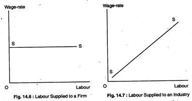
The market supply curve of labour is simply the summation of individual supply curves of labour. Having developed the demand for labour, we now turn to the supply of labour. By adding supply to the analysis, we will be able to find the equilibrium wage-rate. The supply curve of labour, like any supply curve, would be upward-sloping, in a particular industry.

But in a perfectly competitive industry, the individual firm can hire any number of workers at a going wage-rate. Thus, we can say that the industry faces an upward-sloping supply curve but the individual firm faces a horizontal supply curve as in Figs. 14.6 and 14.7.

Theory of Distribution # 35. Labour Leisure Choice and Individual Labour Supply:

All work involves an opportunity cost. As such, analysing the individual decision about how much to work is similar to analysing the consumer’s decision about what to buy in the product market. In fact, the individual is choosing between leisure and the consumption of commodities. A decision to increase the consumption of goods necessarily means a decision to reduce the consumption of leisure.

In order to make a decision, an individual must know the opportunity cost of leisure. That opportunity cost is best represented by the wages (£4) that could have been earned. A decision to work four hours less represents a decision not to be able to consume £16 worth of commodities.

Consider the effect of an increase in wages. The worker is given an incentive to work more because leisure is more expensive. Therefore, the worker substitutes in favour of work and against leisure. This is known as substitution effect of an increase in wages. Looking only at the substitution effect, any increase in wages will cause the worker to want to work longer hours.

But there is also an income effect and it works in the opposite direction. A higher wage-rate means that, for any given number of hours worked, the worker has a greater income. With a greater income, the worker will tend to purchase more of every good, including leisure. Thus, a wage increase tends to reduce the number of hours worked as the worker reduces work efforts.

Generally, the substitution effect outweighs the income effect so that the individual labour supply curve is upward-sloping. Eventually, at a high enough wage-rate, the income effect may dominate, so that, at a sufficiently higher wage-rate the number of hours worked may, in fact, be reduced, at which point it would be backward-binding.

In Fig. 14.8, this backward- bending supply curve of labour shows that, up to wage-rate W₁, the income effect outweighs the substitution effect.

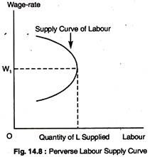
This analysis can be conducted in terms of income leisure choice.

Theory of Distribution # 36. Demand for a Factor:

A profit-maximising firm produces output up to the point where MC = MR. This means that a firm will hire units of the variable factors of production up to the point where MRP (MPP x MR) or VMP (MPP x P of the product) = MFC. Note that a profit-maximising competitive firm will hire additional units of its variable factor up to the point at which MRP (-VMP) = MFC. This is the theory of MP.

In addition, if we assume that labour is the variable factor and that the firm purchases it in a perfectly competitive labour market then MFC will be wage-rate. The theory of MP then states that the firm will hire additional units of labour up to the point at which W = MRP = VMP.

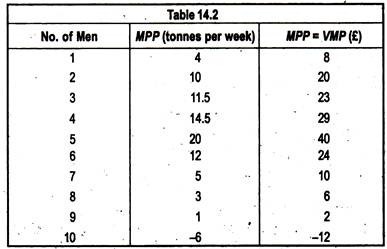
For example, Table 14.2 illustrates the case of a wheat farmer who is operating in perfectly competitive factor and product markets and whose only variable factor of production is labour. Columns (1) and (2) illustrate the “law of diminishing returns” — because when more and more workers are employed, the MPP eventually declines.

Suppose, now, the price of wheat is given as £2 per tonne. This helps us to calculate the MRP (= VMP), which is shown in Column (3) and, since the wage rate is constant, it follows that this must also, eventually, decline as more and more workers are hired.

Thus, the general rate for profit-maximisation is that profit-maximising firms will hire additional units of the variable factors up to the point at which the last unit hired adds just as much to revenue as to cost; that is, until the factors MRP = MFC. This is the equilibrium condition for a profit-maximising firm.

If a firm purchases its variable factor in a perfectly competitive factor market so that it can purchase any quantity without influencing price, the MFC = Price of the factor In this case, the equilibrium condition becomes: MRP – Price of Factor.

This analysis implies that a firm’s MRPC is its demand curve for a variable factor on the assumption that all other factors of production are held constant. Suppose, now, that labour is the only variable factor which is sold in a perfect market.

A profit-maximising firm will employ additional workers up to the point where the wage-rate = MRP. If the weekly wage W= £24, the farmer will maximise profits by employing 6 men, as the MRP of the 6th man equals £24.

The farmer would stop hiring more labour as MFC > MRP. Now assume that the weekly wage falls to £6. In this case, the farmer would employ 8th worker where MRP = wage-rate. Fig. 14.10 represents the above argument where it shows the MRP (=VMP) curve of a profit-maximising firm that Sells its product in a perfect market.

Assume that the firm is able to hire any number of workers at the market wage, so that it faces a perfectly elastic supply curve of labour (S₁S₁) at the market wage (OW). A profit-maximising firm will employ OL₁ units of labour, where, MRP = wage-rate.

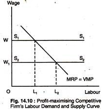
Now, consider the quantity of labour the firm will employ if the wage-rate falls to OW₁ and the supply curve shifts down to S₂S₂. With employment of OL₁ now MRP > the wage-rate, so that firm will hire additional workers. The MRP = wage-rate where again if the firm employs OL₁ units of labour.

Thus, for this firm, its MRP (= VMP) curve represents its demand for labour curve. If, however, the producer is selling the product in an imperfect market, the MR < AR = P. In this case, MRP < VMP.

Theory of Distribution # 37. Equilibrium in a Competitive Factor Market:

A competitive factor market is in equilibrium when the price of the factor input equates the quantity demanded to the quantity supplied.

Fig. 14.11 shows such an equilibrium for a labour market.

The equilibrium wage-rate is. W_C, and the equilibrium employment (where demand equals supply) is L_C .Since they are well-informed, all workers receive identical wages and generate their identical MRP_L, whenever they are employed. If any worker had a wage lower than his MP, a firm would find it profitable to offer that worker a higher wage.

If the output market is also perfectly competitive, the demand curve for the input measures the benefit that consumers of the product place on the additional use of the input in the production process. The wage-rate also reflects the cost to the firm and to society of using an additional unit of the input. Thus, at A in Fig. 14.11(a), the marginal benefit of an hour of labour (MRP_L) is equal to its marginal cost (the wage-rate, W).

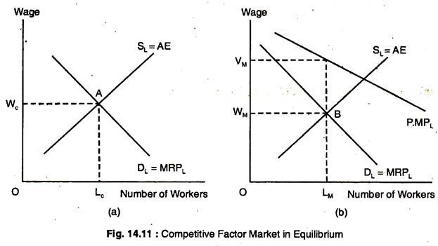
When output and input markets are both perfectly competitive, resources are used efficiently because the difference between total benefits and total costs is maximised where MRP_L = (P)(MP_L). Efficiency requires that the additional revenue received by the firm from employing an additional unit of labour equal the social benefit of the additional output that labour unit produces.

When the output market is not perfectly competitive, the condition MRP_L = (P)(MP_L) no longer holds, which Fig. 14.11(b) shows. The curve representing the product price multiplied by the MP_L lies above the MRP_L[(MR)(MP_L)]. Point B is the equilibrium wage, VK_M and the equilibrium labour supply, L_M. But P. MP_L is the value that consumers place on additional inputs of labour.

Thus, when L_M labourers are employed, the MC to the firm, W_M, is less than the marginal benefit to society, V_M. The firm is maximising its profit, but because its output is less than the efficient level of output, the firm’s input use is also less than the efficient level. Net benefits would increase if the firm hired more factor inputs and, thereby, increase output.

Theory of Distribution # 38. Limitations of the MP Theory:

This theory ignores the supply side, it cannot be regarded as a complete theory of factor pricing. It assumes that labour is a homogenous factor because of differing innate characteristics and skills and labour markets are by no means perfectly competitive.

The theory is based on the assumption that firms attempt to maximise profits. But firms may have other objectives. In such cases, the theory is unlikely to be an adequate explanation of the demand for labour.

The theory also assumes that large level of wages and labour productivity are independent. This is not necessarily valid. Increased wages may increase productivity. Finally, in some countries, it is possible that higher wages may result in more productive workers in the long- run. Such changes in productivity increase the MPP, and, thus, shift a firm’s MRPC to the right.

Theory of Distribution # 39. Imperfection in Labour Market:

Labour markets are really imperfect. On the demand side, there are product monopolies, monopsonies (monopoly buyers of labour) and collusive oligopolies (CBI). On the supply side, there are trade union monopolies which have developed the well-known institution of collective bargaining.

Now we will examine the case of a product monopolist and that of a monopsonistic buyer of labour on the supply side; we consider the influence of trade union and collective bargaining.

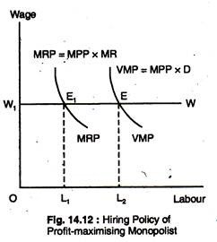
Theory of Distribution # 40. Hiring Policy of a Profit-Maximising Monopolist:

A monopolist faces a downward-sloping demand curve for the good he is producing. This means that if he employs additional workers, he must lower the price of additional output. As shown in Fig. 14.12, the MRPC < the VMPC, because the monopolist’s MRC < ARC.

Assume that the monopolist is operating in a perfectly competitive labour market and, so, faces an infinitely elastic supply curve of labour, WW, paying a fixed wage-rate, OW, per hour as in Fig. 14.12. Thus, such a monopolist will employ OL₁ units of labour, as indicated by the intersection of MRP with WW at point E₁.

Employment of extra units of labour beyond OL₁ would mean that the wage bill would increase in total revenue, thus, reducing profits. OL₁ < OL₂, which would be achieved under conditions of perfect competition in all markets. Thus, monopolist employs less labour than a perfect competitor.

Theory of Distribution # 41. Monopsony Employer of Labour:

Sometimes there could be a monopoly employer of labour, known as monopsony. In these circumstances, the employer may well be able to get the required amount of labour for lower wages, because, employees have no alternative.

This would be most likely if geographical mobility was a serious problem. The monopsonist equilibrium level of employment will be influenced by the MC of labour (called Marginal Expenditure) and the MRP of labour (MRP = VMP). The MC of labour exceeds its AC (=AE).

In Fig. 14.13, the upward-sloping supply curve, SS_L, is in fact the AC (=AE) of labour (AFC). It shows the wage-rate that has to be offered to attract a given supply of labour. Given that the monopsonist is a profit-maximiser, then the number of workers he is willing to employ will be determined by the intersection of MC (= ME) with the MRP = VMP.

The monopsonist employs Oh* units of labour (MEP = MRP). The wage- rate, OW* is given by the intersection of the line EL* with SS_L at point F. Contrast this outcome with the perfectly competitive case when a higher wage-rate, OW_c, and level of employment, OL, would prevail.

Sometimes a monopoly can be created by an employers’ association. Bilateral monopoly exists in the labour market when a single employer or employers’ association negotiates with a single union which covers all the employees in the industry.

Theory of Distribution # 42. Factor Markets with Monopoly Power:

Just as buyers of inputs can have monopsony power, sellers of inputs can have monopoly power. The most important example of monopoly power in the factor markets involves labour unions and we will concentrate most of our attention there. We will briefly describe how a labour union might increase the well-being of its members and substantially affect non-unionized workers.

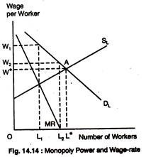
Theory of Distribution # 43. Monopoly Power over the Wage-Rate:

Fig. 14.14 shows that when the seller of a Wage labour input (a labour union) is a monopolist, it per Worker chooses among the points on the buyers’ demand for labour curve, D_L. The seller can maximise the number of workers hired, at L* by agreeing that workers will work at wage, W*.

The quantity of labour, L₁, that maximises the rent, that employees earn, is determined by the intersection of the MR and the supply of labour curves; union members will receive a wage-rate of W₁. Finally, if the union wishes to maximise total wages paid to workers, it should allow L₂ union members to be employed at a wage-rate of W₂ because the marginal revenue to the union will then be zero.

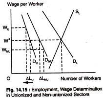
A Two-sector Model of Labour Employment: Wage Determination in Unionized and Non-unionized Sectors:

Fig. 14.15 shows, when a monopolistic union succeeds in raising the wage in the unionized sector of the economy from W* to W_U, employment in that sector falls, as shown by the movement along the demand curve, D_U. For the total supply of labour, S_L, to remain unchanged, the wage in the non- unionized sector must fall from W* to W_NU, as shown by-the movement along the demand curve D_NU.

Theory of Distribution # 44. Bilateral Monopoly in the Labour Market:

Bilateral monopoly is a market in which a monopolist union sells to a monopsonist employer. In a labour market, bilateral monopoly arises when representatives from a union and companies that hire a type of labour meet to negotiate wages. Figure 14.16 shows a typical bilateral bargaining situation.

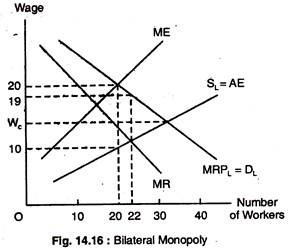
The S_L represents the supply curve of labour, and the firm’s demand curve, for labour is given by the MRP curve D_L. If the union had no monopoly power, the monopsonist would hire 20 workers and pay £10 per hour. When 20 workers are hired, the MRP of labour is equal to the ME of the firm.

The seller of labour faces a demand curve, D_L that describes the firm’s hiring plans as the wage-rate varies. The union chooses a point on the demand curve that maximises its members’ wages, while the supply curve, S_L, tells the union the minimum payment necessary to encourage workers to offer their labour.

Suppose the union wishes to maximise the economic rent of its members; so the union considers the supply curve as the MC of labour. To maximise rent, the union chooses a wage of £19 which equates the MR with MC. At £19, the firms will hire 22 workers.

In summary, the union will demand a wage of £19 and wants firms to hire 22 workers, whereas, firms are willing to offer a wage of £19 and hire 20 workers. What eventually happens depends on the bargaining strategies of the two parties.