
Here is a term paper on the ‘Game Theory’ for class 9, 10, 11 and 12. Find paragraphs, long and short term papers on the ‘Game Theory’ especially written for school and college students.
Term Paper on the Game Theory
Term Paper Contents:
- Term Paper on the Introduction to Game Theory
- Term Paper on the Prisoner’s Dilemma: A Dominant Strategy
- Term Paper on the Bertrand Paradox
- Term Paper on the Inter-Temporal Dimensions
- Term Paper on the Folk Theorem
1. Term Paper on the Introduction to Game Theory:
ADVERTISEMENTS:
Game theory is widely used in different subjects. The use of game theory is increasing day after day because of complexities in economic gains. In mathematics, game theory is used to explain the relationship between the variables. The decision tree is derived to understand the gains from any game. Game theory are of individuals, groups, firms. Every individual is an economic agent in nature. At every point of game, individual expects some economic gains out of different actions.
The agents or firm get benefit to move ahead, collude or disagree with opposite party in the game. Equal benefit to both parties is Nash equilibrium. It can be explained differently as follows. Game theory is a theory of decision making under conditions of uncertainty and interdependence. In game theory, human behavior is studied in strategic situation and a mathematic mode is captured. A strategic game consists of a set of players, which may be a group of nodes or an individual node.
A set of actions for each player to make a decision and preferences over the set of action profiles for each player. In any game utility represents the motivation of players. Applications of game theory always attempt to find equilibriums. If there is a set of strategies with the property that no player can make profit by changing his or her strategy while the other players keep their strategies unchanged, then that set of strategies and the corresponding payoffs constitute the Nash equilibrium.
2. Term Paper on the Prisoner’s Dilemma: A Dominant Strategy:
ADVERTISEMENTS:
The Prisoners’ Dilemma is usually defined between two players. Game Theory assumes that the both players act rationally. Realistic investigations of collective behavior, however, require a multi-person model of the game that serves as a mathematical formulation of what is wrong with human society. The study may lead to a better understanding of the factors stimulating or inhibiting cooperative behavior within social systems. It recapitulates characteristics fundamental to almost every social intercourse. Various aspects of the multi-person Prisoners’ Dilemma have been investigated in the literature.
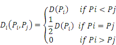
The prisoner’s dilemma gives the dominant strategy. Dominant strategy is an important to study the player’s strategy. It is a dominant strategy in terms of the other player’s strategy. For the purpose, we use the notation; S-Smita is the combination of strategies of every player’s except player Smita. The Player i’s best response or best reply to the strategies S-i, chosen by, the other players. At the same time s*i is the best strategy chosen by ith player that yields him the greatest payoff.
It is written as follows:
![]()
Above notation explains that the best strategy (s*i) has highest gain. The individual choose the best strategies which are dominant strategies. Therefore the dominant strategies are the equilibrium strategies. Such equilibrium strategies are the best response to other player. The dominant strategy does not exist in the welfare game. In the welfare game, there are no dominant strategies. The players work out others actions as the best strategies. The government welfare programs include NREGA in India. The work is sanctioned under this program is to provide the benefits to rural poor people.
ADVERTISEMENTS:
Prisoner’s dilemma is based on certain assumptions:
1. Prisoners Dilemma is a two person game. There are many person’s interacting with each other.
2. We assumed that there is no communication between the two prisoners. If they communicate and commit to co-ordinate then the outcome will be different.
In Prisoners Dilemma, two Prisoners interact only once. Suppose Smita and Deepa are the prisons. If both of them have done the crime and caught by police then they have number of strategies. If Smita and Deepa confess then each is sentenced to ten years in prison. But they are given a choice to confess and deny. Both Smita and Deepa deny of their involvement in crime then both are sentenced to two year in prison. Here there is chance to apply prisoner’s dilemma.
If Smita confesses then she would be released. At the same time, Deepa would be sentenced for 15years in prison. Prisoner’s Dilemma is two by two games. This is because two players will play two different actions and both will try to get more benefit out of their decision. Both have different strategies as confess, deny etc.

Smita and Deepa have their own dominant strategy. Deepa does not know what action is chosen by Smita. If Deepa chooses the action deny, Smita faces the payoff deny and if she confess then she will face payoff 0. Suppose Deepa chooses confess then she will face deny payoff by Smita of 15. Suppose she confesses then payoff is 10. In the above example, Deepa is not better off with confessing. She gets 0 payoffs. The dominant strategy in the above example is confessed, confess. The equilibrium payoff for both the players is (10, 10). But both Deepa and Smita deny then they get (2, 2) same payoffs.
If the equilibrium is dominant strategy then information set does not matter. Suppose Deepa is allowed to confess or deny then Smita move before taking decision is unchanged. The prisoner’s dilemma is useful in various economic theories. It is used in oligopoly pricing, auction bidding, salesman efforts, political bargaining and arms races. Game theory and examples are unrealistic to many scholars. They do not encounter with such kind of incidence. Sometimes thinking in terms of game theory is also important.
ADVERTISEMENTS:
We need to understand strategies and players at different points. A common observation in experiments involving finite repetition of the prisoners’ dilemma is that players do not always play the single-period dominant strategies (finking), but instead achieve some measure of cooperation. Yet finking at each stage is the only Nash equilibrium in the finitely repeated game.
We show here how incomplete information about one or both players’ options, motivation or behavior can explain the observed cooperation. Specifically, we provide a bound on the number of rounds at which Fink may be played, when one player may possibly be committed to a “Tit-for-Tat” strategy.
Types of Games:
There are different types of games in game theory. The co-operative, non-cooperative, welfare, dominant strategy and repeated strategies games are more useful games and we need to understand the behavior of agents.
ADVERTISEMENTS:
Co-Operative and Non Co-Operative Game:
In the co-operative game, the players can make the commitment to each other. Sometimes they go beyond that commitment. It is opposite in the non-cooperative game. In the non-cooperative game, players are not binding for their commitments. All games in the co-operative form are based on principal of Pareto optimality, fairness, and equity. Most of the non-co-operative games are economic in their nature. The players are maximizing their utility subject to stated constraints. The co-operative game theory focuses on properties of the outcome rather than on the strategies.
Such strategies often achieve by the outcome. The co-operative game is used to model bargaining in applied micro economics. Such game is more appropriate than the non-cooperative game. The Prisoners dilemma is a non-cooperative game. Such model can be allowed for players not only to commitment but to make binding constraints. Co-operative games often allow players to split the gains from co-operative games. It is often allow players to split the gains from co-operative by making side payments.
There are following example which shows the different types of games:
ADVERTISEMENTS:
i. A Co-Operative Game without Conflict:
The members of a workforce choose equally heavy tasks to undertake to best co-ordination with each other. It is worked out unity in workforce even though they have diverse strategies.
ii. Co-Operative Game with Conflict:
The game where workforce has different strategies but common strategies are found and it is worked out that there is co-operation among them.
iii. A Non-Co-Operative Game with Conflict:
The Prisoners Dilemma is the best example. Here two players have different strategies. Such strategies remain independent from each other.
ADVERTISEMENTS:
iv. A Non-Co-Operative Game without Conflict:
Two companies set a product standard without communication with each other.
Repeated Dominance: The Battle of the Bismark Sea:
It means a strategy combination found by deleting a weak dominant strategy from the alternative strategy. One of the players recalculating to find which remaining strategy are weakly dominated. Deleting one of them and continuing the process until only one strategy remain for each player.
When people interact over time, threats and promises concerning future behavior may influence current behavior. Repeated games capture this fact of life, and hence have been applied more broadly than any game theoretic model not only in virtually every field of economics but also in finance, law, marketing, political science and sociology.
We have given the example of the battle of Bismarck Sea. The battle of the Bismarck Sea is an example given in the repeated dominance strategies. It is a set in the south pacific in 1943. The General Imamura has been ordered to transport Japanese troops across the Bismarck Sea to New Guinea.
ADVERTISEMENTS:
But General Kenney wants to bomb the troops transport. It is his strategy and chosen at this point. In order to do this, Imamura must choose between a shorter northern route to a longer southern route to new Guineo and Kenney must decide where to send his planes to look for Japanese. Now there are alternative strategies are planned. Suppose Kenny serials his planes to the wrong route he can recall them but the number of days of bombing is reduced.
In the example, the players are Kenney and Imamura and they each have the same action set {North, South}. Their payoffs are never the same. Imamura loses exactly what Kenney gains.
Such game is presented in the following form:

In the above game neither Kenney nor Imamura has a dominant strategy. Kenney would choose North if he thought Imamura would choose North. But at South if he thought Imamura would choose north. There is policy dilemma faced by both players. Suppose he thought Kenney would choose south and he would be indifferent between actions if he thought Kenney would choose north. But we can find a plausible reasonable, probable equilibrium, using the concept of weak dominance.
Suppose strategy Si is weakly dominated then there exists some other strategy S*i for players i. It is possible better yielding a higher payoff in some strategy combination. It never yields a lower payoff. Mathematically, S’i is weakly dominated if there exists S”i such that
![]()
![]()
One might define a weak dominant strategy equilibrium means the strategy profile found by deleting all the weakly dominated strategies of each player. Weakly dominated strategies do not help much in the Battle of the Bismarck Sea. However Imamura’s strategy of South is weakly dominated by the strategy North because his payoff from North is never smaller than his payoff from South. It is greater if Kenney picks South. For Kenney, however, neither strategy is even weakly dominated.
Kenney decides that Imamura will pick North and this is because it is weakly dominant. Therefore Kenney eliminates it. Imamura chooses South from considering such options. Having deleted of column of table Kenney has a strong dominant strategy: he chooses North which achieves payoffs strictly greater than south. The strategy combination (North, North) is an iterated dominant equilibrium and indeed (North, North) was the outcome in 1943.
If Imamura moved first (North, North) then it would be the only equilibrium which is important about a player. This is because he is moving first and it gives the other player more information before he acts. Suppose Kenney has cracked the Japanese code and found Imamura’s plan then there is information leak and both players can move simultaneously. The Battle of the Bismarck Sea is special because the payoffs of the players always sum to zero. This feature is important enough to deserve a name.
A Zero Sum Game:
A zero sum game is a game in which the sum of the payoffs of all the players is zero, whatever strategies they choose. If the game is not zero sums then it is variable sum. In a zero sum game, what one player gains another player must lose. From the above example, the repeated dominance strategy: the Battle of the Bismarck Sea is an example of zero sum game. But the Prisoner’s Dilemma game is not an example of such game. It is not possible to change the payoffs and make the zero sum game. For this, there is need to change the essential character of the games.
ADVERTISEMENTS:
Nash Equilibrium:
Nash equilibrium is standard equilibrium concept in the modern micro-economics. It is widely used concept in various microeconomic models. Suppose the model does not assume specific equilibrium concept but it is used then as Nash or some refinement of Nash equilibrium. Nash equilibrium is a certain kind of rational expectations equilibrium. Nash equilibrium is a situation in which each player chooses an optimal strategy given the strategy chosen the other player.
In Nash equilibrium, each player’s strategy choice is a best response to the strategy choice. It is a best response to the strategies actually played by his rivals. The strategy combination S* is a Nash equilibrium. Suppose player has no incentive to deviate from his strategy then he has incentive to deviate from his strategy given that the other players do not deviate.
![]()
Suppose, one child and adult is asked to stand at box with special panel at one end and a food dispenser at the other. Adult person has strong dominant strategy to get the food whereas the child has weak dominant strategy. Suppose the adult gets to the dispenser first then the child will get only his leaving worth 1 unit. Suppose a child arrives first he eats more units of food and if both arrive at same time then the child get less units of food.

Above brackets shows no dominant strategy equilibrium. It is because what adult will choose depends on what he thinks that the child will choose. Suppose the adult believes that the child will press the panel. The adult will wait by the dispenser. But adult believe that the child would wait and then he would press. There does exist an iterated dominance equilibrium (press, wait).
We will use a different line of reasoning to justify such outcomes. Above example shows the strategy combination (press, wait) is a Nash equilibrium. The way to approach Nash equilibrium is to propose a strategy combination. It is required to test weather each player’s a best response to the others strategy.
Suppose adult picks press and the child faces choice between payoff 2 from pressing and 8 from waiting. At the same time, if adult is willing to wait and child picks wait then the adult has a choice between a payoff of 8 from pressing and 0 from waiting. This confirms that press wait is Nash equilibrium and in fact it is the unique Nash equilibrium.
Such Nash equilibrium is either weak or strong. The weak Nash equilibrium is an inequality strict. It is required that no player be indifferent between his equilibrium strategy and some other strategy. Every dominant strategy is Nash equilibrium but not every Nash equilibrium dominant strategy is equilibrium. Suppose the strategy is a dominant strategy then it is a best response to any strategies that the other players pick. It includes their equilibrium strategy. If a strategy is part of a Nash equilibrium if need only a best response to the other players.
3. Term Paper on the Bertrand Paradox:
Bertrand paradox was developed in 1883. It is an extension of the Cournot model. Bertrand paradox model is based on assumptions and they are explained as follows.
Assumption:
(i) Two firms produce identical goods which are “non-differentiated”. Such goods are perfect substitutes in the consumer’s utility function.
(ii) Consumers buy from the producer who charges the lowest price.
(iii) Each firm faces a demand schedule which is equal to half of the market demand at the common prices.
(iv) Firms always supply commodities as the demand it faces.
The market demand function is q = D (p)
Each firm incurs a cost c per unit of production. The profit of firm i is
![]()
Where, the demand for output of firm i is denoted Di. It is given by
The aggregate profit is defined as
![]()
![]()
Such aggregate profit cannot exceed the monopoly profit
![]()
![]()
Each firm can guarantee itself a non-negative profit. It is possible by charging a price above the marginal cost. Therefore the profits of the firm is explained as
![]()
The firm chooses their prices both simultaneously and non-co-operatively. A Nash equilibrium in prices sometimes referred to as a Bertrand equilibrium. It is a pair of prices (P*1, P*2). Each firm’s price maximizes that firm’s profit given the other firms price. Formally, for all i = 1, 2 and
For all pi
![]()
The Bertrand (1883) paradox states that the unique equilibrium and two firms charge the competitive price.
![]()
The proof is as follows
Consider for example
![]()
The firm one has no demand and its profit is zero. On the other hand if firm one charges
![]()
Now ε is positive and small. It obtains the entire market demand, D(P2* – ε) and has a positive profit margin of
![]()
Therefore firm one cannot be acting in its own best interest if it charges P1*.
Now suppose that
![]()
Then the profit of firm one is
![]()
If firm one reduces its price slightly to P1* ⎯ ε its profit becomes
![]()
It is greater for small. In above situation, the market share of the firm increases in a discontinuous manner. This is because no firm will charge less than the unit cost C. The lowest price firm would make a negative profit. We are left with one or two firms charging exactly c. In order to show that both firms do charge c. Suppose
![]()
The firm two which makes no profit and it could raise its price slightly. But still it can supply all the demand and make a positive profit- a contradiction.
The conclusion of this simple model is as follows. We have written it in points:
i. That firm’s price is at marginal cost.
ii. That firms do not make profits
We call these two situations as Bertrand Paradox because it is hard to believe that firms in industries with never succeed in manipulating.
Market Price to Make Profits:
In a symmetric case conclusion I and II do not hold, indeed the following can be shown:
i. That both firms charges price p = c2, and
ii. That firm 1 makes a profit of (c2-c1) D (c2) and firm 2 makes no profit.
Thus firm 1 charge above marginal cost and makes a positive profit. The Bertrand equilibrium is no longer welfare-optimal. But again , the conclusion is a bit strained firm one makes very little profit if C2 is close to c1 and firm two makes no profit at all.
Solution to Bertrand Paradox:
In the above model, we have made three crucial assumptions. Now in order to prove the Bertrand paradox, we need to relax one assumption from the above there assumptions.
The Edge Worth Solution:
The Edge worth solved the Bertrand paradox in 1897. He solved the Bertrand paradox by introducing capacity constraints by which firms cannot sell more than they are capable of producing. To understand this idea, suppose that firm one has a production capacity smaller than D(c.) The equilibrium is (Pi*,P2*) = (c, c). It is still an equilibrium price system. At this price both firm makes zero profit.
Suppose that firm two increases its price slightly then firm one faces demand D(c) but it cannot satisfy. The rational way is that some consumers must move to firm two. Firm two has a nonzero demand. It is at price greater than its marginal cost therefore it makes positive profit. Consequently, the Bertrand solution is no long term equilibrium. The general rule is that the models with capacity constraints, firms make positive profit. The market price is greater than the marginal cost.
4. Term Paper on the Inter-Temporal Dimensions:
The second crucial assumption in the above model is that one shot game. It does not always seem to reflect economic reality as it stands. In the Bertrand solution, the equilibrium is P1 = P2 > C. But it is not an actual equilibrium in the model.
The answer is that firm one for example could benefit from a slight decrease in its price (i.e. to P ⎯ õ) and from its resulting takeover of the entire market. Nothing happens after that because of Bertrand’s crucial assumption of one short game. In reality, firm two would probably decrease its price in order to regain its share of the market. If we introduce this temporal dimension and the possibility of reaction, it is no longer clear that firm one would benefit from decreasing its price below P2.
Firm one would have to compare the short run gain (the rise of its market share) to the long run loss in price war.
Sub Game Perfectness:
The perfect equilibrium of follow the leader I:
Sub game perfectness is an equilibrium concept based on the ordering of moves and the distinction between an equilibrium path and equilibrium. The equilibrium path is the path through the game tree that is followed in equilibrium, but the equilibrium itself is a strategy combination. It includes the player’s responses to other player’s deviations from the equilibrium.
The path perfectness is a way to eliminate some of the weak Nash equilibrium. A flow of Nash equilibrium was revealed in the game follow the leader I, which has three pure strategies. Nash equilibrium is one of the reasonable strategies. The players are Smita and Deepa, who choose disk sizes.
Both their payoffs are greater if they choose the same size and greatest if they co-ordinate on the size Large. Smita moves first so her strategy becomes more complicated. Although, she must specify an action for each information set, Deepa’s information set depends on what Smita chooses. Deepa’s strategy set is large and small. It specifies that she chooses large if smita chooses large. She chooses small if Smita choose small.
We found the following three Nash equilibriums:
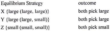
From the above outcomes equilibrium Y is reasonable strategy for both players. This is because the order of the moves should matter to the decision players. The problem with the normal form and thus with simple Nash equilibrium is that it ignores who moves first. Smita’s moves first and it seems reasonable that Deepa should be allowed. In fact she should be required to rethink her strategy after Smita’s moves.

Now consider Deepa’s equilibrium Z strategy of Small, Small. If Smita deviated from equilibrium and she is choosing large then it would be unreasonable for Deepa to stick to the response of large. She would indeed choose large and Z would not be equilibrium. A similar case shows that (Large, Large) is an irrational strategy for Deepa and we are left with Y as the unique equilibrium. We say that equilibrium X and Z are Nash equilibrium. But they are not “Perfect” Nash equilibrium.
A strategy combination is a perfect equilibrium if it remains equilibrium on all possible paths both the equilibrium path and their paths which branch of into different sub games. A sub game is a game consisting of a node which is a singleton in every player information partition that nodes successor. A strategy combination is a sub game perfect Nash equilibrium if (a) it is Nash equilibrium for the entire game and (b) its relevant action rules are Nash equilibrium for every sub game.
The extensive form of follow the Leader I has three sub games:
(i) The entire game
(ii) The sub-game starting at node B1
(iii) The sub-game which is starting at node B2
Strategy combination x is not a sub-game perfect equilibrium because it is only Nash in sub-games (1) and (3). But it is not Nash equilibrium in sub-game 2. The strategy combination Z is not a sub-game perfect equilibrium. It is because only Nash in sub-games (1) and (2) is not in sub- game (3). But strategy combination Y is Nash in all three sub-games.
One reason why perfectness is a good concept is because out at equilibrium behavior is irrational in a non-perfect equilibrium. A second justification is that a weak Nash equilibrium is not robust to small changes in the game.
An example of Perfectness Entry Deterrence I:
In this game, we assume that there are two players. The first firm is the new entrant firm and the other is senior firm. The information is perfect and uncertain.
There are two actions and events observed in this game:
(i) The new entrant firm decides whether to enter or stay out
(ii) If the entrant enters the senior can collude with him or fight by cutting the price drastically.
Following are the payoffs to both in this game:
Market profits are 100 at the monopoly price and 0 at the fighting price entry costs 10 collusion shares the profits evenly.
The strategy sets can be discovered from the order of actions and events. They are {enter, stay out} for the entrant and {collude if entry occurs, fight if entry occurs} for the senior firm. The game has the two Nash equilibrium indicated in bold face (enter, collude) and (stay out, fight). The equilibrium (stay out, fight) is weak because the senior would just as soon collude given that the new entrant is staying out.

Once he has chosen enter, the senior firm’s best response is collude. The threat to fight is not credible and would be employed only if the senior could bind himself to fight in which case he never does fight. It is because the new entrant chooses to stay out. The equilibrium (stay out, fight) is Nash but not sub-game perfect because if the game is started after the new entrant has already entered the senior best. Response is colluding. This does not prove that collusion is inevitable in duopoly but collusion is the equilibrium for entry deterrents-I

Suppose there is effective communication between the two players then the game will change. The senior firm might tell the new entrant that entry would be followed by fighting. But the new entrant would ignore this non-credible threat. Suppose senior could pre commit himself to fight entry, the threat would become credible. A game in which a player can commit himself to a strategy then it can be modeled in two ways.
Firstly as a game in which non-perfect equilibrium are acceptable. Secondly, we assume that by changing the game to replace the action of both the players. The second approach is better than first. This is because usually the modeler wants to let players commit to some actions and not others. Player can do this by carefully specifying the order of play. Allowing equilibrium to be non-perfect forbids such discrimination and usually multiplies the number of equilibriums.
Sub game perfectness is too restrictive and it still allows too many strategy combinations to be equilibrium in games of asymmetric information. A sub game must start at single node and it should not cut across any player’s information set. It is often the only sub-game which will be the whole game and imposing sub-game perfectness. It does not restrict equilibrium at all.
5. Term Paper on the Folk Theorem:
It is part of the conventional wisdom of game theory that threats of mini-max punishments. It can sustain any individually rational collusive allocation as Nash equilibrium of an infinitely repeated game. Games in which players meet in strategic interactions repeatedly are referred to as repeated games. It is not possible to assign authorship of the result. It is known as the worst. The firm being punished is making its best response to the action of the punisher.
In an infinitely repeated n person game with finite action sets at each repetition any combination of actions observed in any finite number of repetitions. It is the unique outcome of some sub-game perfect equilibrium.
The three conditions are given and they are explained in detail as follows:
Condition 1:
The rate of time perfectness is zero or positive and sufficiently small.
Condition 2:
The probability that the game ends at any repetition is zero or positive and sufficiently small and
Condition 3:
The set of payoff combinations that, strictly Pareto dominates. The mini-max payoff combinations in the mixed extension of, the one ⎯ short game has n dimensions.
The folk theorem explains that particular behavior arises in a perfect equilibrium. It is meaningless in an infinitely repeated game. This applies to any game that meets condition one to three which we saw in above paragraph. If an infinite amount of time always remained in any game, a way can be found to make one player willing to punish some other player for the sake of better future.
It is even if the punishment currently hurts the punisher as well as punished. Any infinite interval of time is in-significant; it is compared to infinity. The threat of future reprisal makes the players willing to carry out the punishments needed. It is most practical example observed in the industry.
The folk theorem has emerged as the best theorem in modern microeconomics. It implies that in repeated games any outcomes are a feasible solution concept. Under that outcome, the player’s mini-max conditions are satisfied. The mini-max condition states that a player will minimize the maximum possible loss. An outcome is said to be feasible if it satisfies this condition for each player of the game. A
repeated game is one in which there is not a final move but there is a sequence of round. Each player may gather information and choose moves. In mathematics, the theorem is believed and discussed but it has not been published.
A grim trigger strategy is a strategy which punishes an opponent for any deviation from some certain behavior. Therefore all players of the game must have a certain feasible outcome. The players need only adhere to an almost grim trigger strategy. Any deviation from the strategy will bring about the intended outcome.
It is punished to a degree that any gains made by the deviator on account of the deviation are exactly cancelled out. Thus, there is no advantage to any player for deviating from the course which will bring out the intended and arbitrary outcome. The game will proceed in exactly the manner to bring about that outcome.
Following conditions are important for our understanding:
Condition1: Discounting:
We know that with discounting the present gain from confessing is weighted more heavily. The future gains from co-operation are taken more lightly. If the discounting rate is very high the game almost returns to being one shot. Suppose the real interest rate is high then a payment next year is little better than a payment a hundred years later. Therefore next year is practically irrelevant.
Any model that relies on a large number of repetitions also relies on the discount rate not being too high. The alarming strategy imposes the heaviest possible punishment for prisoner’s dilemma. For consumer goods the discount is given because short terms gains are more as compare to long term. There are more innovations possible in long term.
Condition 2: A Probability of the Game Ending:
Time preference is fairly straight forward. The assumption is that the game ends each period with probability Q. There are different examples where game ends with time. It does not make a drastic, difference if Q > 0. The probability of game ending is taken as one or it is put less than expected number of repetition. It is still behaving like a discounted game. This is because the expected number of future repetitions is always large. It is no matter how many have already occurred. We always believe that there is end of each game.
The following two situations are different of each other:
i. The game will end at some uncertain data before T. In statistics, it is assumed as T.
ii. There is a constant probability of the game ending.
iii. Under the game theory, each game is like a finite game. This is because as time passes the maximum amount of time still to run shrinks to zero, even though the game will probably end T. If it lasts until T, the game looks exactly the same as at time zero.
Condition 3: The Dimensionality Condition:
The mini-max payoff is the payoff of the result. Suppose all the other players pick strategies solely to punish players i then he protects himself as best he can. There are different methods of risk diversions. The dimensionality condition is need for games with three or more dimension. It is satisfied if for each game which has same payoff. The desired behavior requires some way to the other players to punish a deviator, without punishing themselves. It is observed in terms of different dimensions in game.