Term Paper on the Elasticity of Demand | Economics

Here is a compilation of term papers on the ‘Elasticity of Demand’ for class 11 and 12. Find paragraphs, long and short term papers on the ‘Elasticity of Demand’ especially written for commerce students.

1. Term Paper on the Price Elasticity of Demand:

Price elasticity of demand indicates the degree of responsiveness of quantity demanded of a good to the change in its price, other factors such as income, prices of related commodities that determine demand are held constant. Precisely, price elasticity of demand is defined as the ratio of the percentage change is quantity demanded to a percentage change in price.

Thus,

It follows from the above definition of price elasticity of demand that when percentage change in quantity demanded a commodity is greater than the percentage change in price that brought it about, price elasticity of demand (e_p) will be greater than one and in this case demand is said to be elastic.

On the other hand, when a given percentage change in price of a commodity leads to a smaller percentage change in quantity demanded, elasticity will be less than one and demand in this case is said to be inelastic. Further, when the percentage change in quantity demanded of a commodity is equal to the percentage change in price that caused it, price elasticity is equal to one.

Thus in case of elastic demand, a given change in price causes quite a large change in quantity demanded. And in case of inelastic demand, a given change in price brings about a very small change in quantity demanded of a commodity.

It is a matter of common knowledge and observation that there is a considerable difference between different goods in regard to the magnitude of response of demand to the changes in price. The demand for some goods is more responsive to the changes in price than those of others.

In terminology of economics, we would say that the demand for some goods is more elastic than those for the others or the price elasticity of demand of some goods is greater than those of the others. Marshall who introduced the concept of elasticity into economic theory remarks that the elasticity or responsiveness of demand in a market is great or small according as the amount demanded increases much or little for a given fall in price, and diminishes much or little for a given rise in price.

This will be clear from Fig. 7.1 and 7.2 which represent two demand curves. For a given fall in price, from OP to OP, increase in quantity demanded is much greater in Fig. 7.1 than in Fig. 7.2. Therefore, demand curve in Fig. 7.1 is more elastic than the demand curve of Fig. 7.2 for a given fall in price for the portion of demand curves considered. Demand for the good represented in Fig. 7.1 is gen­erally said to be elastic and the demand for the good in Fig. 7.2 to be inelastic.

It should, however, be noted that terms elastic and inelastic are used in the relative sense. In other words, elasticity is a matter of degree only. Demand for some goods is only more or less elastic than others. Thus, when we say that demand for a good is elastic, we mean only that the demand for it is relatively more elastic.

Likewise, when we say that demand for a good is inelastic, we do not mean that its demand is absolutely inelastic but only that it is relatively less elastic. In economic theory elastic and inelastic demands have come to acquire precise meanings. Demand for a good is said to be elastic if the price elasticity of demand for it is greater than one.

Similarly, the demand for a good is called inelastic if price elasticity of demand for it is less than one. Price elasticity of demand equal to one, or in other words, unit elasticity of demand therefore represents the dividing line between elastic and inelastic demand. It will now be clear that by inelastic demand we do not mean perfectly inelastic but only that the elasticity of demand is less than unity; and by elastic demand we do not mean absolutely elastic but that the elasticity of demand is greater than one.

Thus,

Elastic demand: e_n > 1

Inelastic demand: e_p < 1

Unitary elastic demand: e_p = 1

Price Elasticity of Demand for Different Goods Varies a Good Deal:

Goods show great variation in respect of elasticity of demand i.e., their responsiveness to changes in price. Some goods like common salt, wheat and rice are very unresponsive to the changes in their prices. The demand for salt remains practically the same for a small rise or fall in its price.

Therefore, demand for common salt is said to be ‘inelastic’. Demand for goods like radios, refrigerators etc., is elastic, since changes in their prices bring about large changes in their quantity demanded. We shall explain later at length those factors which are responsible for the differences in elasticity of demand of various goods.

It will suffice here to say that the main reason for differences in elasticity of demand is the Possibility of substitution i.e., the presence or absence of competing substitutes. The greater the ease with which substitutes can be found for a commodity or with which it can be substituted for other commodities, the greater will be the price elasticity of demand of that commodity.

Goods are demanded because they satisfy some particular wants and in general wants can be satisfied in a variety of alternative ways. For instance, the want for entertainment can be gratified by having television set, or by possessing a gramophone, or by going to cinemas or by visiting theatres.

If the price of a television set falls, the quantity demanded of television sets will rise greatly since fall in the price of television will induce some people to buy televisions in place of having gramophones or visiting cinemas and theatres. Thus the demand for televisions is elastic.

Likewise, if the price of ‘Lux’ falls, its demand will greatly rise because it will be substituted for other varieties of soap such as Jai, Hamam, Godrej, Pears etc. On the contrary, the demand for a necessary good like salt is inelastic. The demand for salt is inelastic since it satisfies a basic human want and no substitutes for it are available. People would consume almost the same quantity of salt whether it becomes slightly cheaper or dearer than before.

Perfectly Inelastic and Perfectly Elastic Demand:

We will now explain the two extreme cases of price elasticity of demand. First extreme situation is of perfectly inelastic demand which is depicted in Fig. 7.3. In this case a change in price of a commodity does not affect the quantity demand of the commodity at all. In this perfectly inelastic demand, demand curve is a vertical straight line as shown in Fig. 7.3.

As will be seen from this figure, whatever the price quantity demanded of the commodity remains unchanged at OQ. An approximate example of perfectly inelastic demand is the demand of acute diabetic patient for insulin. He has to get the prescribed doze of insulin per week whatever its price.

The second extreme situation is of perfectly elastic demand in which case demand curve is a horizontal straight line as shown in Fig. 7.4. This horizontal demand curve for a product implies that a small reduction in price would cause the buyers to increase the quantity demanded from zero to all they could obtain.

On the other hand, a small rise in price of the product will cause the buyers to switch completely away from the product so that its quantity demanded falls to zero. 

Products of different firms working under perfect competition are completely identical. If any perfectly competitive firm raises the price of its product, it would lose all its customers who would switch over to other firms and if it reduces its price somewhat it would get all the customers to buy the product from it.

Measurement of Price Elasticity:

Price elasticity of demand expresses the response of quantity demanded of a good to changes in its price, given the consumer’s income, his tastes and prices of all other goods. Thus price elasticity means the degree of responsiveness or sensitiveness of quantity demanded of a good to a change in its price.

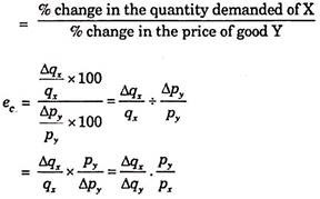
An important method to measure price elasticity of demand is the percentage method. Price elasticity can be precisely measured by dividing the percentage change in quantity demanded in response to a small change in price, divided by the percentage change in price.

Thus we can measure price elasticity by using the following formula:

or, in symbolic terms;

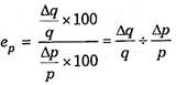
Where,

e_p stands for price elasticity

q Stands for the original quantity

p Stands for the original price

Δ Stands for a small change

Mathematically speaking, price elasticity of demand has a negative sign since the change in quantity demanded of a good is in opposite direction to the change in its price. When price falls, quantity demanded rises and vice versa. But for the sake of convenience in understand­ing the magnitude of response of quantity demanded of a good to a change in its price we ignore the negative sign and take into account only the numerical value of the elasticity.

Thus, if 2% change in price leads to a 4% change in quantity demanded of good A and 8% change in that of B, then the above formula of elasticity will give the value of price elasticity of good A equal to 2 and that of good B equal to 4. It indicates that the quantity demanded of good B changes relatively much more than that of good A in response to a given change in price.

But if we had written minus signs before the numerical values of elasticities of the two goods, that is, if we had written the elasticity as – 2 and – 4 respectively as strict mathematics would require us to do, then since – 4 is smaller than – 2, we would have been misled in concluding that price elasticity of demand of B is less than that of A. But, response of demand for B to the change in its price is greater than that of A, it is better to ignore minus sign and draw conclusion from the absolute values of elasticities. Hence, by convention minus sign before the value of price elasticity of demand is generally ignored in economics.

Arc Elasticity of Demand:

The concept of point elasticity of demand which refers to the price elasticity at a point on the demand curve or, in other words, which refers to the price elasticity when the changes in the price and the resultant changes in quantity demanded are infinitesimally small. In this case if we take the original price and original quantity or the subsequent price and quantity after the change in price as the basis of measurement, there will not be any significant difference in the coefficient of elasticity.

However, when the price change is quite large or we have to measure elasticity over an arc of the demand curve rather than at a specific point on it, the measure of point elasticity, namely Δq/Δp . p/q does not provide us the true and correct measure of price elasticity of demand.

Further, in such cases, the coefficient of price elasticity would be different depending upon whether we choose original price and quantity or the subsequent price and quantity demanded as the basis for measurement of price elasticity and therefore there will be significant difference in the two coefficients of elasticity, obtained from using two bases.

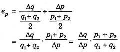
Therefore, when the change in price is quite large, say more than 10 percent, and then accurate measure of price elasticity of demand can be obtained by taking the average of original price and subsequent price as well as average of the original quantity and subsequent quantity as the basis of measurement of percentage changes in price and quantity.

Thus, if price of a good falls from p₁ to p₂ and as a result its quantity demanded increases from q₁   to q₂, the average of the two prices is given by p₁ + p₂/2 and average of the two quantities (original and subsequent) is given by p₁ + p₂/2.

Thus, the formula for measuring arc elasticity, that is, when change in price is quite large is given by:

Methods Used for Calculating the Price Elasticity of Demand:

Let us solve some numerical problems of price elasticity of demand (both point and arc) by percentage method.

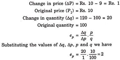
Problem 1:

Suppose the price of a commodity falls from Rs. 10 to Rs. 9 per unit and due to this quantity demanded of the commodity increases from 100 units to 120 units. Find out the price elasticity of demand.

Solution:

Problem 2:

A consumer purchases 80 units of a commodity when its price is Re. 1 per unit and purchases 48 units when its price rises to Rs. 2 per unit. What is the price elasticity of demand for the commodity?

Solution:

It should be noted the change in price from Re. 1 to Rs. 2 in this case is very large (i.e., 100%). Therefore, to calculate the elasticity coefficient in this case arc elasticity formula should be used.

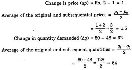
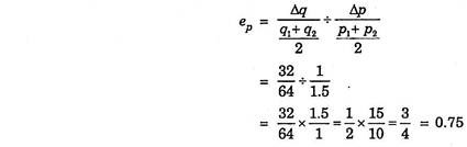
Thus, the price arc elasticity of demand obtained is equal to 0.75.

Problem 3:

Suppose a seller of a textile cloth wants to lower the price of its cloth from 150 per metre to Rs. 142.5 per metre. If it’s present sales are 2000 metres per month and further it is estimated that its elasticity of demand for the product equals – 0.7.

Show:

(a) Whether or not his total revenue will increase as a result of his price; and

(b) Calculate the exact magnitude of its new total revenue.

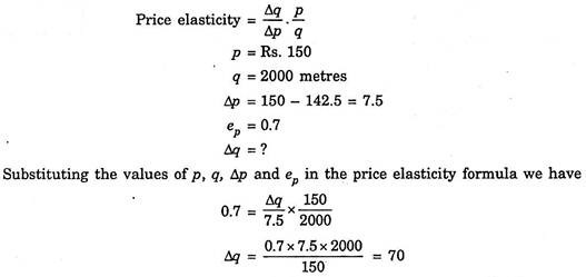
Since price has fallen quantity demanded will increase by 70 metres. So the new quan­tity demanded will be 2000 + 70 = 2070.

(b) Total Revenue before reduction in price = 2000 × 150 = Rs. 3,00,000 Total revenue after reduction = 2070 × 142.5 = Rs. 2,94,975.

Thus with reduction in price his total revenue has decreased.

Total Expenditure or Total Revenue Method:

We have explained above the percentage method of measurement of price elasticity of demand. There is also another method to measure price elasticity of demand. This is known as total expenditure method or total revenue method. The price elasticity of demand for a good and the total expenditure made on the good are greatly related to each other.

From the changes in the total expenditure made on a good as a result of changes in its price, we can know the price elasticity of demand for the good. But it should be remembered that with the total expenditure method we can know only whether elasticity is equal to one, greater than one or less than one. With this method we cannot find out the exact and precise coefficient of elasticity.

Unit Elasticity (e_p = 1):

When as a result of the change in price of a good the quantity demanded of the good increases so much that the total expenditure made on the good remains the same, the elasticity of demand for the good is equal to unity. This is because total expenditure made on a good can remain the same only if the percentage change in quantity demanded is equal to the percentage change in price.

Elasticity Greater Than One (e_p > 1):

When due to the fall in price the quantity demanded of a good increase so much that the total expenditure made on the good in­creases, the price elasticity of demand will be greater than unity. This is so because with a fall in price of a good the total expenditure on it can increase only if the percentage increase in the quantity demanded is greater than the percentage change in price.

It should be carefully noted that when due to the rise in price, the total expenditure on the good declines, elasticity of demand will be greater than one because increase in total expenditure as a result of fall in price and decrease in total expenditure as a result of rise in price are the same things.

Elasticity Less Than One (e_p < 1):

If as a result of fall in the price of the good, the total expenditure on it decreases, the price elasticity of demand will be less than unity. This is because with the fall in price the total expenditure can decrease only if the percentage increase in the quantity demanded of a good is less than the percentage fall in its price. Thus, when due to the rise in price the total expenditure made on the good increases the price elasticity of demand will be less than one.

Illustration of Expenditure Method:

Let us illustrate how we judge the elasticity of demand as to whether it is greater than one, equal to one or less than one. Consider Table 7.1, which gives quantity demanded of pens at various prices. It will be seen from Table 7.1 that quantity demanded increases from 30 pens at price Rs. 5 per pen to 87 pens at price Rs. 3.25.

We have calculated the total outlay by multiplying the quantity demanded with the corresponding price of the pen. It will be observed from the table that when price of the pen falls from Rs. 5 to Rs. 4.75, from Rs. 4.75 to Rs. 4.50, from Rs. 4.50 to Rs. 4.25 and from Rs. 4.25 to Rs. 4, the quantity demanded increases so much that the total outlay on pens increases indicating thereby that elasticity of demand is greater than one at these prices.

When the price falls from Rs. 4.00 to Rs. 3.75, the quantity demanded increases from 75 pens to 80 pens so that total outlay remains the same at Rs. 300. This shows that price elasticity of demand is unity. When the price of the pen further falls from Rs. 3.75 to Rs. 3.50 and then to Rs. 3.25 the total outlay spent on pens decreases. Thus, the elasticity of demand for pens at these prices is less than unity.

Problem 4:

Suppose price of a good falls from Rs. 10 to Rs. 8 per unit. As a result, its quantity demanded increases from 80 units to 100 units. What can we say about price elasticity of demand by total revenue method?

Solution:

At price Rs. 10, quantity demand is 100 units.

Therefore, total revenue at price Rs. 10 = P × Q = 10 × 80 = Rs. 800

At the lower price Rs. 8, quantity demand increases to 100 units.

Therefore, total revenue at price Rs. 8 = P × Q = 8 × 100 = Rs. 800

We thus find that with the change in price of the good, total revenue of the firm remains constant. Hence price elasticity of demand is equal to one.

Graphic Illustration of Expenditure Method:

This relationship between the price elasticity of demand and total outlay can also be graphically illustrated with the aid of the demand curve. This relationship between price elasticity of demand and total expenditure, made on good is illustrated with the aid of Fig. 7.5 where demand curve DD is given. In the Fig. 7.5 when the price is OP, the total expenditure made on the good is equal to OP × OQ i.e., area OPRQ and when the price falls to OP’, the total expenditure is equal to OP’R’Q’.

It will be seen from the Figure 7.5 that the area OP’HQ is common in both the rectangles OPRQ and OP’R’Q’. Now, by comparing the remaining areas PRHP and QHR’Q’ we find that two are equal to each other. That is, the total outlay OP’R’Q’ is equal to the original outlay OPRQ. This means that with the fall in price the total outlay (expenditure) made on the good has remained the same. Hence the price elasticity of demand is here equal to unity.

That when the price elasticity of demand is greater than one, the total expenditure made on the good increases with the fall in the price of the good is illustrated in Fig. 7.6 in which a demand curve DD is given. When the price of the good is OP, OQ quantity of the good is demanded. At the price of OP, the total expenditure made on the good is equal to the area OPRQ.

Now, if price of the good falls to OP’, the quantity demanded of the good rises to OQ’. Therefore, now at price OP total expenditure on the good is equal to the area OP’R’Q’. It will be seen in Fig. 7.6 that the area OP’HQ is present in both the rectangles OPRQ and OP’R’Q’. The remaining areas sin the two rectangles are PRHP’ and QHR’Q’.

Now, a glance at Fig. 7.6 will show that the area QHR’Q’ is greater than the area PRHP’. It is thus clear that the expenditure (OP’R’Q’) on the good at price OP’ is greater than the expenditure (OPRQ) at price OR, that is, with the fall in price the total expenditure has increased. Hence, the price elasticity of demand is here greater than unity.

Now, consider Fig. 7.7. In this figure the demand for the good is such that with the fall in price the total expenditure made on the good declines. At price OP the total expenditure is OPRQ and when the price falls to OP the total expenditure made on it is equal to OP’R’Q’. Now, by comparing the two total expenditures it is evident that the expenditure OP’R’Q’ is less than the expenditure OPRQ. Therefore, the price elasticity of demand is here less than unity.

From the above analysis it is clear that from the changes in the total expenditure as a result of the changes in price we can know the price elasticity of demand for a good. We repeat once again that with the total expenditure method we cannot know the exact and precise measure of the price elasticity; with this we can only know whether price elasticity is equal to one, greater than one or less than one.

Measuring Price Elasticity of Demand:

Measurement of Price Elasticity of Demand at a Point on the Demand Curve:

Let a straight line demand curve DD’ is given and it is required to measure price elasticity at a point R on this demand curve. It will be seen from Fig. 7.8 that corresponding to point R on the demand curve DD’, price is OP and quantity demand at it is OQ.

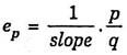
The measure of price elasticity of demand is given by:

The first term in this formula, namely Δp/Δq . p/q the reciprocal of the slope of the demand curve DD (Note that the slope of the demand curve DD’ is equal Δq/Δp which remains constant all along the straight line demand curve). The second term in the above point elasticity formula is the original price (p) divided by the original quantity (q).

Thus,

It will be seen from Fig. 7.8 that at point R, original price p = OP and original quantity q = OQ. Further, slope of the demand curve DD’ is Δp/Δq .PD/PR.

Substituting these values in the above formula we have:

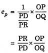
A glance at Fig. 7.8 reveals that PR = OQ and they will cancel out in the above expression.

Therefore,

Measuring price elasticity by taking the ratio of these distances on the vertical axis, that is, OP/PD is called vertical axis formula.

In a right angled triangle ODD’, PR is parallel to OD.

Therefore:

RD’ is the lower segment of the demand curve DD’ at point R and RD is its upper segment.

Therefore:

Measuring price elasticity at a point on the demand curve by measuring the ratio of the distances of lower segment and upper segment is another popular method of measuring point price elasticity on a demand curve.

Measuring Price Elasticity on a Non-Linear Demand Curve:

If the demand curve is not a straight line like DD’ in Fig. 7.8 but is, as usual, a non-linear curve, then how to measure price elasticity at a given point on it. For instance, how price elasticity at point R on the demand curve DD’ in Fig. 7.9 is to be found. In order to measure elasticity in this case, we have to draw a tangent TT’ at the given point R on the demand curve DD’ and then measure price elasticity by finding out the value of RT’/RT.

On a Linear Demand Curve Price Elasticity Varies From Zero to Infinity:

Now again, take the straight-line demand curve DD’ (Fig. 7.10). If point R lies exactly at the middle of this straight-line demand curve DD’, then the distance RD will be equal to the distance RD’. Therefore, elasticity which is equal to RD’/RD will be equal to one at the middle point of the straight-line demand curve.

Suppose a point S lies above the middle point on the straight-line demand curve DD’. It is obvious that the distance SD’ is greater than the distance SD and price elasticity which equal to SD’/SD at point S will more than one. Similarly, at any other point which lies above the middle point on the straight-line demand curve, price elasticity will be greater than unity.

Moreover, price elasticity will go on increasing as we move further towards point D and at point D elasticity will be equal to infinity. This is because price elasticity is equal RD’/RD i.e., Lower segment/upper segment and as we move towards D the lower segment will go on increasing while the upper segment will become smaller.

There­fore, as we move towards D on the demand curve, the price elasticity will be increasing. At point D, the lower segment will be equal to the whole DD’, and the upper segment will be zero. Therefore, Price elasticity at point D on the demand curve DD’ = DD’/0 = infinity.

Now, suppose a point L lies below the middle point on the linear demand curve DD’. In this case, the lower segment LD’ will be smaller than the upper segment LD and therefore price equal elasticity at L which is to LD’/LD will be less than one.

Moreover, elasticity will go on decreasing as we move towards point D’. This is because whereas lower segment will become smaller and smaller, the upper one will be increasing as we move towards point D’. At point D’ the elasticity will be zero, since at D’ the lower segment will be equal to zero and the upper one to the whole DD’.

At point D’

e_p = 0/DD’= 0

Price Elasticity Varies at Different Points on a Non-Linear Demand Curve:

From above it is clear that elasticity at different points on a given demand curve (or, in other words, elasticity at different prices) is different. This is not only true for a straight- line demand curve but also for a non-linear demand curve. Take, for instance, demand curve DD in Fig. 7.11. Elasticity at R on the demand curve DD will be found out by drawing a tangent to this point. Thus elasticity at R will be RT’/RT. Since distance RT’ is greater than RT, price elasticity at point R will be more than one.

How exactly it is, will be given by actual value which is obtained from dividing RT’ by RT. Likewise, price elasticity at point S will be given by SJ’/SJ. Because SJ’ is smaller than SJ, elasticity at S will be less than one. Again how exactly it is, Quantity will be found from actually dividing SJ’ by SJ. It is thus evident that elasticity at point S is less than that at point R on the demand curve DD. Similarly, elasticity at other points of the demand curve DD will be found to be different.

Comparing Price Elasticity of Two Demand Curves:

Having explained the concept of price elasticity of demand we will now explain how the compare elasticity on two demand curves. First, we take up the case of two demand curves with different slopes starting from a given point on the Y-axis. This case is illustrated in Fig. 7.12 where two demand curves DA and DB which have different slopes but are starting from the same point D on the Y-axis. Slope of demand curve DB is less than that of DA.

Now, it can be proved that at any given price the price elasticity on these two demand curves would be the same. If price is OP, then according to demand curve DA, OL quantity of the good is demanded and according to demand curves DB, OH quantity of the good is demanded. Thus, at price OP the corresponding points on the two demand curves are E and F respectively. We know that price elasticity at a point on the demand curve is equal to Lower segment/upper segment.

Therefore, the price elasticity of demand at point E on the demand curve DA is equal to EA’/ED and the price elasticity of demand at point F on the demand curve DB is equal to EB/FD.

Now, take triangle ODA which is a right-angled triangle in which PE is parallel to OA. It follows that in it, EA/ED is equal to PD. Thus, the price elasticity at point E on the demand curve DA is equal to OP/PD.

Now, in the right-angled triangle ODB, PF is parallel to OB. Therefore, in it FB/FD is equal to OP/PD. Thus, price elasticity of demand at point F on the demand curve DB is also OP/PD. From above it is clear that price elasticity of demand on points E and F on the two demand curves respectively is equal to OP/PD, that is, elasticities of demand at points E and F are equal PD though the slopes of these two demand curves are different. It follows therefore that the elasticity is not the same thing as slope. Therefore, price elasticity on two demand curves should not be compared by considering slope alone.

Comparing Price Elasticity on Two Intersecting Demand Curves:

We now take up the case of comparing price elasticity at a given price when the two demand curves intersect. In Fig. 7.13 we have drawn two demand curves AB and CD which intersect at point E. It will be noticed from the figure that demand curve CD is flatter than the demand curve AB.

Now, it can be easily proved that at every price, on the flatter demand curve CD, price elasticity will be greater than that on the relatively steeper demand curve AB. For example at price OP, corresponding to the intersecting point E, using the vertical axis formula, elasticity at point E on demand curve CD = OP/PC.

Similarly, elasticity at point E on the demand curve AB = OP/PA. It will be seen from Fig. 7.13 that OP/PC > OP/PA because distance PC is less than the distance PA. Hence at the price OP, elasticity is greater on the flatter demand curve CD, as compared to steeper demand curve AB. Likewise, it can be shown at any other given price, and elasticity of demand will be greater on the flatter demand curve CD as compared to the steeper demand curve AB.

Comparing Price Elasticity on Two Parallel Demand Curves:

Now, we will compare the price elasticity at two parallel demand curves at a given price. This has been illustrated in Fig. 7.14 where two demand curves AB and CD are given which are parallel to each other. The two demand curves’ being parallel to each other implies that they have the same slope. Now, we can prove that at price OP price elasticity of demand on the two demand curves AB and CD is different. Now, draw a perpendicular from point R to the point P on Y-axis. Thus, at price OP the corresponding points on the two demand curves are Q and R respectively.

The elasticity of demand on the demand curve AB at point Q will be equal to QB/QA and at point R on the demand curve CD it is equal to RD/RC.

Because in a right-angled triangle OAB, PQ is parallel to OB:

Therefore, QB/QA = OP/PA

Hence, price elasticity at point Q on the demand curve:

AB = OP/PA

At point R on the demand curve CD, price elasticity is equal to = RD/RC. Because in the right-angled triangle OCD, PR is parallel to OD.

Therefore, RD/RC = OP/PC.

Hence, on point R on the demand curve CD, price elasticity = OP/PC.

On seeing the diagram it will be clear that at point Q the price elasticity OP/PA and at point R the price elasticity OP/PC are not equal to each other. Because PC is greater than PA, OP/PC = OP/PA.

It is, therefore, clear that at point R on the demand curve CD the price elasticity is less than that at point Q on the demand curve AB, when the two demand curves being parallel to each other have the same slope. It also follows that as the demand curve shifts to the right the price elasticity of demand at a given price goes on declining. Thus, as has been just seen, price elasticity at price OP on the demand curve CD is less than that on the demand curve AB.

Importance of the Price Elasticity of Demand:

The concept of elasticity of demand plays a crucial role in the pricing decisions of the business firms and the Government when it regulates prices. The concept of price elasticity is also important in judging the effect of devaluation of a currency on its export earnings. It has also a great use in fiscal policy because the Finance Minister has to keep in view the elasticity of demand when it considers imposing taxes on various commodities.

We shall explain below the various uses, applications and importance of the elasticity of demand:

1. Pricing Decisions by Business Firms:

The business firms take into account the price elasticity of demand when they take decisions regarding pricing of the goods. This is because change in the price of a product will bring about a change in the quantity demanded depend­ing upon the coefficient of price elasticity.

This change in quantity demanded as a result of, say a rise in price by a firm, will affect the consumer’s total expenditure and will therefore, and affect the revenue of the firm. If the demand for a product of the firm happens to be elastic, then any attempt on the part of the firm to raise the price of its product will bring about a fall in its total revenue.

Thus, instead of gaining from the increase in price, it will lose if the demand for its product happens to be elastic. On the other hand, if the demand for the product of a firm happens to be inelastic, then the increase in price by it will raise its total revenue. Therefore, for fixing a profit maximising price, the firm cannot ignore the price elasticity of demand for its product.

Price elasticity of demand can be used to answer the following types of questions:

1. What will be the effect on sales if a firm decides to raise the price of its product, say by 5 per cent?

2. How large a reduction in price of a product is required to increase sales, say by 25 per cent?

It has been found by some empirical studies that business firms often fail to take elasticity into account while taking decisions regarding prices, or they give insufficient attention to the coefficient of price elasticity. No doubt, the main reason for this is that they don’t have the means to calculate price elasticity for their product, since sufficient data regarding past prices and quantity demanded at those prices are not available.

Even if such data are available, there are difficulties of interpretation of it because it is not clear whether the changes in quantity demanded were the result of changes in price alone or changes in some other factors determining the demand.

However, recently big corporate business firms have established their research departments which estimate the coefficient of price elasticity from the data concerning past prices and quantities demanded. Further, they are also using statistical techniques to isolate the price effect on the quantity demanded from the effects of other factors.

2. Uses in Economic Policy Regarding Price Regulation, Especially of Farm Prod­ucts:

Governments of many countries, especially United States of America, regulate the prices of farm products. This price regulation involves the increase in the prices of farm products, and this is done with the expectation that the demand for the farm products is inelastic.

That the demand for farm products is inelastic in countries like USA has been found from empirical studies. By restricting supply in the market, Government succeeds in raising the price for the farm products. The demand for these products being inelastic, the quantity demanded does not fall very much and as a result the expenditure of the consumers on farm products increases, which raises the incomes of the agricultural class.

If the de­mands for farm products were elastic, any rise in their price brought about by Government’s restricted supply of them, would have caused the decrease in the incomes of the agricultural class. Therefore, the crop restriction programme and keeping part of the crop off the market by the Government would never have been considered, had the demand for farm products been elastic rather than inelastic.

3. Explanation of the ‘Paradox’ of Plenty:

The concept of price elasticity of demand also, helps us to explain the so called ‘paradox of plenty’ in agriculture, namely, that a bumper crop reaped by the farmers brings a smaller total income to them. The fall in the income or revenue of the farmers as a result of the bumper crop is due to the fact that with greater supply the prices of the crops decline drastically and in the context of inelastic demand for them, the total expenditure on the crop output declines, bringing about fall in the incomes of the farmers.

Thus, bumper crop instead of raising their incomes reduces them. Therefore, in order to ensure that the farmers do not lose incentive to raise their production, they need to be assured certain minimum price by the Government. At that minimum price the Government should be prepared to buy the crop from the farmers.

4. Use in International Trade:

The concept of price elasticity of demand is also crucially important in the field of international economics. The Governments of the various countries have to decide about whether to devalue their currencies or not when their exports are stagnant and imports are mounting and as a result their balance of payments position is worsening.

The effect of the devaluation is to raise the price of the imported goods and to lower the prices of the exports. If the demand for a country’s exports is inelastic, the fall in the prices of exports as a result of devaluation will lower their foreign exchange earnings rather than increasing them. This is because, demand being inelastic, as a result of the fall in prices quantity demanded of the exported products will increase very little and the country would suffer because of the lower prices.

On the other hand, if the demand for a country’s exports is elastic, then the fall in the prices of these exports due to devaluation will bring about a large increase in their quantity demanded which will increase the foreign exchange earnings of the country and will thus help in solving the balance of payments problem. Thus, the decision to devalue or not, depends upon the coefficient of the demand elasticity of exports.

Likewise, if the objective of devaluation is to reduce the imports of a country, then this will be realised only when the demand for the imports is elastic. The imports will decline very much as a result of rise in their prices brought about by devaluation and the country will save a good amount of foreign exchange.

On the other hand, if the demand for imports is inelastic, the increase in prices as a result of devaluation will adversely affect the balance of payments, because at higher prices of the imports and almost the same quantity of imports, the country would have to spend more on the imports than before.

5. Importance in Fiscal Policy:

The elasticity of demand is also of great significance in the field of fiscal policy. The Finance Minister has to take into account elasticity of demand of the product on which he proposes to impose the tax if the revenue for the Government is to be increased. The imposition of an indirect tax, such as excise duty or sales tax, raises the price of a commodity.

Now, if the demand for the commodity is elastic, the rise in price caused by the tax will bring about a large decline in the quantity demanded and as a result the Government revenue will decline rather than increase. The Government can succeed in increasing its revenue by the imposition of commodity taxes only if the demand for the commodity is inelastic.

The elasticity of demand also determines to what extent a tax on a commodity can be shifted to the consumer. Thus, the incidence of a commodity tax on the consumers depends on their elasticity of demand for the commodity. If the demand for a commodity is perfectly inelastic, the whole of the burden of the commodity tax will fall on the consumers. When a tax is imposed on a commodity, its price will rise.

As in the case of perfectly inelastic demand, the quantity demanded for the commodity remains the same, whatever the price, the price will rise to the extent of the tax per unit. Therefore, the consumers will bear the whole burden of the tax in the form of a higher price they pay for the same quantity demanded.

On the contrary, if the demand for a commodity is perfectly elastic, the imposition of the tax on it will not cause any rise in price and, therefore, the whole burden of the tax will be borne by the manufacturers or sellers. When demand is neither perfectly inelastic, nor perfectly elastic, then respective burdens borne by the consumers and the producers will depend upon the elasticity of demand as well as on the elasticity of supply. We thus see that a Finance Minister cannot ignore elasticity of demand for products while levying taxes.

2. Term Paper on the Cross Elasticity of Demand:

Very often demands for two goods are so related to each other that when the price of any of them changes, the demand for the other good also changes, when its own price remains the same. Therefore, degree of responsiveness of demand for one good in response to the change in price of another good represents the cross elasticity of demand of one good for the other.

The concept of cross elasticity of demand is illustrated by Fig. 7.15 where demand curves of two goods X and Y are given. Initially, the price of good Y is OP₁ at which OQ₁ quantity of it is demanded and the price of good X is OP at which OM₁ quantity of it is demanded.

Now suppose that the price of good Y falls from OP₁ to OP₂, while price of good X remains constant at OP. As a consequence of the fall in price of good Y from OP₁ to OP₂, its quantity demanded rises from OQ₁ to OQ₂. In drawing the demand curve, D_xD_x for good X, it is assumed that the prices of other goods (including good Y) remain the same.

Now that the price of good Y has fallen and as a result its quantity demanded has increased, it will have an effect on the demand for good X. If good Y is a substitute for good X, then as a result of the fall in price of good Y from OP to OP₂, the demand curve of good X will shift to the left, that is, the demand for good X will decrease.

This is because as the quantity of good increases, the marginal utility of its substitute good declines and therefore the entire mar­ginal utility curve of the substitute good shifts to the left. As shall be seen from the Fig. 7.15 that as a result of the fall in price of good Y, the demand curve of good X shifts from D_x D_x to the dotted position D’_x D’_x so that at price OP now less quantity OM₂ of X is demanded. M₁M₂ of good X has been substituted by Q₁ Q₂ of good Y.

It should be noted that if good X instead of being substitute is complement of good Y, the resultant increase in its quantity demand of good Y due to fall in its price would have caused the increase in demand for good X and a result the entire demand curve of good X, instead of shifting to the left, would have shifted to the right. This is because when the price of a good falls and consequently its quantity demanded increases, the marginal utility of its complement would increase and therefore its entire demand curve would shift to the right.

With a rightward shift of the demand curve of good X, the greater quantity of it will be demanded at the given price OP.

It should be noted again that in the concept of cross elasticity of demand, while the price of one good changes, there is a change in the quantity demanded of another good.

When the quantity demanded of good X falls as a result of the fall in the price of good Y, the coefficient of cross elasticity of demand of X for Y will be equal to the percentage change in the quantity demanded of good X in response to a given percentage change in the price of good Y.

Therefore:

Coefficient of cross elasticity of demand of X for Y

Where,

e_c stands for cross elasticity of demand of X for Y

Q_x stands for the original quantity demanded of X

Δq stands for change in quantity demanded of good X

p_y stands for the original price of good Y

ΔP_y stands for a small change in the price of good Y

Problem 5:

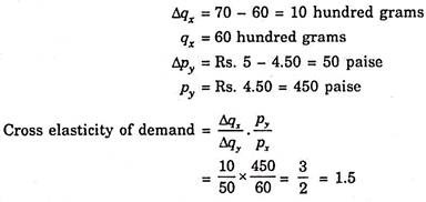
Let us take an example. If the price of coffee rises from Rs. 4.50 per hundred grams to Rs. 5 per hundred grams and as a result the consumer’s demand for tea increases from 60 hundred grams to 70 hundred grams, then the cross elasticity of demand of tea for coffee can be found out as follows.

In the above example:

Substitute and Complementary Goods:

As we have seen in the example of tea and coffee above, when two goods are substitutes of each other, then as a result of the rise in price of one good, the quantity demanded of the other good increases. Therefore, the cross elasticity of demand between the two substitute goods is positive, that is, in response to the rise in price of one good, the demand for the other good rises.

Substitute goods are also known as competing goods. On the other hand, when the two goods are complementary with each other just as bread and butter, tea and milk etc., the rise in price of one good brings about the decrease in demand for the other.

Therefore, the cross elasticity of demand between the two complementary goods is negative. Therefore according to the classification based on the concept of cross elasticity of demand, goods X and Y are substitutes or complements according as the cross elasticity of demand is positive or negative.

The concept of cross elasticity of demand is very important in economic theory. The substitute and complementary goods, are defined in terms of cross elasticity of demand. The goods between which cross elasticity of demand in positive are known as substitute goods and the goods between which cross elasticity of demand is nega­tive are complementary goods.

Besides, classification of various types of market structures is made on the basis of cross elasticity of demand. Thus, Professor Triffen has employed the concept of cross elasticity of demand in distinguishing the various forms of markets. Perfect competition is defined as that in which the cross elasticity of demand between the products produced by many firms in it is infinite.

Monopoly is said to exist when a producer produces a product the cross elasticity of demand for which with any other product is very low. In fact, the pure or absolute monopoly is sometimes defined as the production by a single producer of a product whose cross elasticity of demand with any other product is zero. Monopolistic competition is said to prevail in the market when a large number of firms produces those products between which cross elasticity of demand is large and positive, that is, they are close substitutes of each other.

Importance of Cross Elasticity of Demand for Business Decision Making:

The concept of cross elasticity of demand is of great importance in managerial decision making for formulating proper price strategy. Multiproduct firms often use this concept to measure the effect of change in price of one product on the demand for other products. For example, Maruti Udyog Ltd. produces Maruti Vans, Maruti 800 and Maruti Esteem.

These products are good substitutes of each other and therefore cross elasticity of demand between them is very high. If Maruti Udyog decides to lower the price of Maruti 800, it will signifi­cantly affect the demand for Maruti Vans and Maruti Esteem. So it will formulate a proper price strategy fixing appropriate price for its various products.

Further, Gillete Company produces both razors and razor blades which are complements with high cross elasticity of demand. If it decides to lower the price of razors, it will greatly increase the demand for razor blades. Thus there is need for adopting a proper price strategy when it produces products with high positive or negative cross price elasticity of demand.

Second, the concept of cross elasticity of demand is frequently used in defining the boundaries of an industry and in measuring interrelationship between industries. An indus­try is defined as a group of firms producing similar products that is, products with a high positive cross elasticity of demand. For example cross elasticity of demand between Maruti Esteem, Dawoo Ceilo, and Opel Astra is positive and quite high.

They therefore belong to the same industry (i.e., automobiles). It should be noted that because of interrelationship of firms and industries between which cross price-elasticity of demand is positive and high, any one cannot raise the price of its product without losing sales to other firms in the related industries.

Further, the concept of cross elasticity of demand is extremely used in the United States in deciding cases relating to antitrust laws and monopolistic practices used by firms. It so happens that in order to reduce competition that one dominant firm producing a product with high cross elasticity of demand with the products of other firms tries to take over them and thereby establish a monopoly or different firms try to merge with each other to form a cartel to enjoy monopolistic profits.

These actions are held illegal by Antitrust or anti- monopoly laws. An interesting attempt was made in India by Coca-Cola. In 1995 when it returned to India following the adoption of policy of liberalisation. In order to reduce com­petition, Coca-Cola company purchased the firm producing Thums Up, Gold Spot, Limca which have high positive cross elasticity of demand with Coca-Cola and it further made efforts to take over ‘Pure Drinks’, the producer of Campa-Cola, another close substitutes but failed. If it had succeeded in its venture it could have significantly reduced competition. With this its competition would have been with other multinational rival firm Pepsi-Cola.

3. Term Paper on the Income Elasticity of Demand:

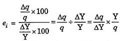
Another important concept of elasticity of demand is income elasticity of demand. In­come elasticity of demand shows the degree of responsiveness of quantity demanded of a good to a small change in the income of consumers. The degree of response of quantity demanded to a change in income is measured by dividing the proportionate change in quantity demanded by the proportionate change in income. Thus, more precisely, the income elasticity of demand may be defined as the ratio of the percentage change in purchases of a good to a percentage change in income which induces the former.

Let Y stand for an initial income, ΔY for a small change in income, Δq for the initial quantity purchased, Δq for a change in quantity purchased as a result of a change in income and e_t for income elasticity of demand.

Then,

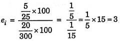
If, for instance, consumer’s weekly income rises from Rs. 300 to Rs. 320, his purchase of the good X increases from 25 units per week to 30 units, then his income elasticity of demand for X is:

Income elasticity of demand being zero is of great significance. Zero income elasticity of demand for a good implies that a given increase in income does not at all lead to any increase in quantity demanded of a good or expenditure on it. In other words, zero income elasticity signifies that a quantity demanded of the good is quite unresponsive to changes in income.

Income Elasticity, Normal Good and Inferior Goods:

Besides, zero income elasticity is significant because it represents dividing line between positive income elasticity on the one side and negative income elasticity on the other. On the one side, when income elasticity is more than zero (that is, positive), then an increase in income leads to the increase in quantity demanded of the good. This happens in case of normal goods.

On the other side of zero income elasticity are all those goods whose income elasticity is less than zero (that is, negative) and in such cases increase in income will lead to the fall in quantity demanded of the goods. Goods having negative income elasticity are known as inferior goods. Goods with positive income elasticity are called normal goods. We thus see that zero income elasticity is a significant value, for it helps us to distinguish normal goods from inferior goods.

Income Elasticity, Luxuries and Necessities:

Another significant value of income elasticity is unity. This is because when income elasticity of demand for a good is equal to one, then proportion of income spent on the good remains the same as consumer’s income increases. Income elasticity of unity also represents a useful dividing line. If the income elasticity for a good is greater than one, the proportion of consumer’s income spent on the good rises as consumer’s income increase, that is, that good bulks larger in consumer’s expenditure as he becomes richer.

On the other hand, if the income elasticity for a good is less than one, the proportion of consumer’s income spent on it falls as his income rises, that is, the good becomes relatively less important in consumer’s expenditure as his income rises. A good having income elasticity more than one and which therefore bulks larger in consumer’s budget as he becomes richer is called a luxury.

A good with an income elasticity less than one and which claims declining proportion of consumer’s income as he becomes richer is called a necessity. It should, however, be noted that the definitions of luxuries and necessities on the basis of income elasticity may not conform to their definitions in English dictionary because the dictionary’s luxuries may be necessities and its necessities may be luxuries according to the above definition. But in economic theory it is useful to call the goods with income elasticity greater than one as luxuries and goods with income elasticity less than one as necessities.

Importance of Income Elasticity for Business Firms:

The concept of income elasticity is important for decision making both by business firms and industries. First, the firms producing products which have high income elasticity have great potential for growth in an expanding economy. For example, if for a firm’s product income elasticity of demand is greater than one; it means that it will gain more than proportionately to the increase in national income.

Thus firms which are producing products having high income elasticity are more interested in forecasting the level of aggregate economic activity (i.e., level of national income) because the demand for their products will greatly depend on the level of overall economic activity. Further, as seen above, the demand for luxuries is highly income elastic. Therefore, the demands for luxuries fluctuate very much during different phases of business cycles. During boom periods, demand for luxuries in­crease very much, and decline sharply during recessionary periods.

On the other hand, the demand for products with low income elasticity will not be greatly affected by the fluctuations in aggregate economic activity. During booms the demand for their products will not increase much and during recessions it will not decrease sharply. Therefore, the firms with low income elasticity for their products would not be much inter­ested in forecasting future business activity. Remember it is generally necessities for which demand is not much income elastic.

However, there is one good thing for the firms which face low income elasticity. They are to a good extent recession-proof. In the periods of recession, their incomes do not fall to the extent of decline in aggregate income. Of course, to share the benefits of increasing national income firms currently producing products with low income elasticity would try to enter the industries demand for whose products is highly income elastic as this would ensure better growth opportunities.

The knowledge of income elasticity of demand also plays a significant role in designing marketing strategies of the firms. If income of people is an important determinant of demand for a product, the firms producing product with high income elasticity of demand will be located in those areas or set up their sales outlets in those cities or regions where incomes are increasing rapidly. Besides, the firms will direct their advertising campaigns and other sales production activities to those segments of people whose income is high and also in­creasing rapidly. This is to ensure higher growth of sales of their products.

The concept of income elasticity of demand shows clearly why farmers income do not rise equal to that of urban people engaged in manufacturing industries. Income elasticity of demand for agriculture products such as food-grains is less than one. This implies that it is difficult for the farmers’ income from agriculture to increase in proportion to the expand­ing national income. Thus farmers cannot keep up with the urban people who derive their incomes from industries producing goods with high income elasticity of demand.