Rate of Interest— General Equilibrium

Read this article to learn about the problem, determinate theory, schedules and their shifts in general equilibrium of rate of interest.

The Problem:

Between loanable funds and liquidity preference theory—which one to choose and why?

Prof. J.R. Hicks has described such a dispute as a ‘sham dispute’, for the neo-classical (loanable funds) formulation and the Keynesian formulation, taken together, do supply us with an adequate and determinate theory of the rate of interest.

Since both the classical theory of the rate of interest and the Keynesian theory go to determine the rate of interest at a given level of income; both of them taken separately are indeterminate because one is unable to know the rate of interest, unless one knows the given level of income and one cannot know the giver, level of income unless one knows the rate of interest; thus both the theories are indeterminate. The determinate theory, on the other hand, emphasizes the fact that the two approaches are just two aspects of the more general approach in which income and the rate of interest are determined simultaneously.

For this purpose an economy is broadly divided into two sectors—the ‘monetary sector’ and the ‘goods sector’. An increase in the quantity of money may be spent in the ‘commodity market’, thereby raising income to a point at which the excess cash becomes the desired cash needed for transactions ; or the extra cash may be used to purchase securities etc., thereby reducing the rate of interest until the excess cash is willingly held as an idle balance. In other words, the two (monetary and commodity) sectors are inter- related; but for the general equilibrium of the economy they must also be separately in equilibrium.

For the equilibrium of the ‘monetary sector’ rate of interest and the level of income must be such that the supply of money equals the demand for it (M = L). The commodity sector is in equilibrium if the rate of interest and the level of income are such that they equate savings and investment (S = I). Thus, an equilibrium or determinate rate of interest is one which brings about simultaneous general equilibrium in the monetary as well as in the goods sector (at an equilibrium level of income when the multiplier process has worked itself out).

In fact, when we talk of the determination of the equilibrium or determinate rate of interest, what we have in mind is the determination of the equilibrium level of income (because both the rate of interest and income are simultaneously determined). We have seen that the changes in the quantity of money affect both income and the rate of interest. But quantity of money is only one determinant of income and rate of interest.

Other determinants are:

(i) The investment demand schedule,

(ii) The consumption function,

(ii) The liquidity preference schedule.

These three, together with the quantity of money as fixed by the monetary authority, determine together the level of income and the rate of interest. Put in the conventional terminology we may restate the proposition as follows:

There are four determinants of income and the rate of interest:

(i) Productivity,

(ii) Thrift,

(iii) Desire for cash,

(iv) The quantity of money.

An equilibrium condition (income) is reached when the desired volume of cash (L) equals the quantity of money (M), when the MEC is equal to the rate of interest; and finally, when the volume of investment is equal to the normal or desired volume of saving (i.e., L = M, r = MEC, S = I and, therefore, Y = C + I). All these factors are inter-related.

Let us study analytically the inter-relationship of these factors:

Determinate Theory:

The classical or neo-classical formulation of loanable funds does not give us a determinate theory of the rate of interest. It treats productivity and thrift as essential elements in any theory of interest but it doesn’t tell us how the rate of interest gets determined. It throws no light on the most crucial question— whether the rate of interest is a determinant of the system or the determinate? All that loanable funds formulation gives us a family of loanable funds schedules (or saving schedules in the Keynesian-Pigovian Sense) at various income levels—showing how much people will save at different rates of interest and different levels of income. In Fig. 22.1 they are shown as S₁(Y₁), S₂(Y₂), S₃(Y₃) etc.

The shape of these schedules implies that people will save more at higher rate of interest than at low rates. The fact that there are different schedules for different assumed levels of national income shows the classicals belief that people will save more, given the rate of interest, the higher their income. II.

I’I’ are investment demand curves showing how much businessmen would wish to invest at different rates of interest. The position and shape of these schedules depend, among other things, on the physical productivity of capital. The figure is meant to show, not what the rate of interest will be, but what levels of income will be associated with different rates of interest.

Exactly the same criticism applies to Keynesian theory of liquidity preference of the rate of interest. It also fails us as a determinate theory of the rate of interest; because the liquidity preference schedule will change up or down with change in income level, therefore, the theory is equally indeterminate. From the Keynesian formulation what we get is a family of liquidity preference schedules at various income levels and not a theory of the rate of interest.

In Fig. 22.2 each liquidity preference curve is associated with one level of income and shows how the demand for money at that level of income will respond to changes in the rate of interest, with every rise in income, more money is required for ‘transactions’ and to satisfy the ‘precautionary’ motives and the liquidity preference schedule therefore, moves to the right. In Fig. 22.2 L₁, L₂ and L₃ are the liquidity preference schedules at different levels of income. On this family of liquidity preference schedules, we superimpose a schedule of money supply. It is assumed that the money supply is fixed (by the Central Bank) and the money schedule is, therefore, a straight vertical line. Fig. 22.2, thus, contains the essence of the Liquidity Preference Theory.

The LM Schedule:

In the money market the economic activities centre round the demand for and supply of money to hold. These activities are lumped together because they include the different forms in which wealth holders seek to hold economic value over time. The demand for money consists of transactions demand (L_t) and the asset demand (L_a). Therefore, L = L_t + L_a. The money supply also consists of two parts for transaction purposes (M_a) and for holding it as an asset (M_t). Therefore, M = M_t + M_a. Hence, the essential condition for monetary equilibrium is:

L_t + L_a = M_t + M_a.

The total demand for money (L) is a function of both income and the rate of interest and one of its components: (L_t) is a function of income, while the other component, the asset demand (L_a) is a function of the rate of interest. In other words, equilibrium with respect to L_t, is linked to income and equilibrium with respect to L_a is linked to the rate of interest. Therefore, general equilibrium in monetary sector is defined in terms of both income and the rate of interest.

The liquidity preference function L and the money supply M also establish a relation between income and the rate of interest. Given a certain liquidity preference (demand schedule for money) and a certain supply of money fixed by monetary authority, the rate of interest will be low when the income is low and high when the income is high. The curve showing this relation, we call the LM curve.

It is also a functional curve and shows the relation between income and interest (given L function and the supply of M), when the desired cash equals the actual cash, or when L = M. The LM curve presupposes equilibrium between L and M, just as the IS curve presupposes equilibrium between I and S. The LM curve is shown in Fig. 22.3.

The LM curve shows (assuming the money supply rigidly fixed by the monetary authority), that a low level of income will mean a relatively abundant supply of money and so a low rate of interest: a high income will mean a relatively small money supply and so a high rate of interest. At high levels of income, there is large transactions demand for the limited quantity of money, and so the rate of interest rises steeply; the LM curve becomes highly inelastic with respect to the rate of interest at high income levels.

On the other hand, at low income levels, there is a small ‘transactions demand’ for the fixed quantity of money, and so a large part of the money may be held as an idle balance; the effect is to lower the interest rate. The LM curve at low income levels is interest elastic.

There is a limit to the extent that the rate of interest can fall, because the asset demand function becomes perfectly elastic at relatively low rates of interest. This is the liquidity trap. Once we reach the critical level at which interest-rates do not respond to further increases in the quantity of money for holding idle balances, then LM curve becomes perfectly elastic with respect to the rate of interest.

The dotted curve LM₁ represents a shift in the LM schedule caused by either:

(i) An increase in the quantity of money controlled by the monetary authority or

(ii) A decrease in LP.

Assuming no change in LP, any increase in the quantity of money will shift the LM curve to the right; and similarly, assuming no change in the quantity of money, any decrease in the demand for money (the L function) will ease the situation and tend to lower the rate of interest at any given income level, or conversely raise the level of income consistent with any given rate of interest. Thus, either a decrease in LP or an increase in the quantity of money will shift the LM curve to the right, as shown by LM₁.

The IS Schedule:

We know that the rate of interest, investment and income are all inter-related. Investment is a form of ‘income generating’ expenditure. It creates income not only directly but indirectly also through its effects on consumption. Every given level of investment has a corresponding level of equilibrium income—defined as the level of income attained when the ‘multiplier’ process has worked itself What this equilibrium level of income is, depends on the size of the ‘multiplier’, which in depends upon the MPC).

The fact is that for a given level of investment (= saving) there is a particular and corresponding level of equilibrium income and the rate of interest—this inter-relationship is represented through what Hicks calls the IS curve. The IS curve is a functional curve and shows the relation of income and the rate of interest when the multiplier process has fully worked itself outside investment and savings are then in equilibrium. Savings and investment are always equal; but when the full multiplier effect has been reached are savings and investment in equilibrium. At the point actual savings equal normal savings as determined by the normal marginal propensity to save.

Fig. 22.4 shows income on the horizontal and the rate of interest on the vertical axis. Given a certain marginal efficiency of investment schedule, a high rate of interest will permit only a little investment. This means a low level of income, even where account is taken of the multiplier. At a low rate of interest, however, investment would be larger, and so the level of income (account being taken of the multiplier) will be relatively high. Accordingly, the IS curve slopes downwards to the right. Given the investment function and the consumption function (from which later the multiplier is derived); income is high (OY) at low rates of interest (Or) and low (OY) at high rates of interest (6%).

The IS curve shows the relation. With a rate of interest at 6%, the level of investment will be such that, the MPC being what it is, the equilibrium level of income’ will be OY. The various points on the IS curve show the equilibrium between S and I (given the MEC and MPC), at different rates of interest giving rise to different levels of income. If, however, the investment or the MPC increases due to some reason, the IS curve will shift to the right, I’S’. It means that at the same rate of interest of 6% saving and investment are equalized at a higher level of income OY’.

To repeat the IS curve depends upon the level (and slope) of the MEC (investment function) and equally upon the level (and slope) of MPC (consumption function). An upward movement in MEC or in MPC or both, will raise the level of income corresponding to each rate of interest.

The IS schedule shows the condition of equilibrium in the goods market of a simple economy without government and foreign transactions—the necessary condition for equilibrium is that investment and saving ex-ante be equal. If we introduce G into the analysis but continue to assume that there are no international transactions, the necessary condition for equilibrium becomes one in which ex-ante I + G is equal to ex-ante saving plus net taxes, S + T.

Again if we introduce international transactions, the necessary condition for equilibrium is one, in which, I + G + X = S + T + M. In considering the equilibrium in goods market, it is convenient to assume a closed economy, the basic condition for equilibrium, in which, is ex-ante equality of S + T and I + G. Saving and taxes are a function of income (Y), whereas investment expenditure are an inverse function of the rate of interest, and the government expenditures (G) are assumed to be autonomous with respect to both income and rate of interest.

The General Equilibrium:

The Intersection of IS and LM Curves:

We have now two curves, IS and LM, which relate income and the rate of interest. Neither of them can by itself tell us either the rate of interest or the level of income. We know what the level of income will be, given the rate of interest, but we cannot say what the rate of interest will be unless we know the level of income. But by combining the IS and LM curves, we can determine simultaneously both the rate of interest and income.

This is done in Fig. 22.5. This figure shows that given the MEC and MPC embodied in the IS curve, the supply and demand for money embodied in the LM curve, the rate of interest is determined as i and income Y. This means a macroeconomic (general) equilibrium of economy, in which the monetary and goods sectors are simultaneously in equilibrium. In other words, Oi is that unique rate of interest which brings about equality between saving and investment in the goods market and equality between the demand for and supply of money in the money market, that is. I = S and L = M.

By combining the LM and IS curves in a general model in the Fig. 22.5 we get an understanding of the manner in which the money market and the goods market are linked together. IS and LM curves intersect at a point where income is OY_np and the rate of interest is O₁.

These are equilibrium levels with respect to income and the rate of interest. There are any number of levels of both income and the rate of interest, i.e., that are compatible with equilibrium of either S and I alone, or L and M considered alone, but there is only one unique rate of interest (the interest) and only one unique level of income (the income) that is consistent with equilibrium in both the monetary and goods sectors.

The actual level of both income and interest that is consistent with equilibrium in the two sectors depends on the shape and the level assumed for the LM and IS curves. At the point of intersection of these curves, the output level (Y_np) and the rate of interest (Oi), are such that (S + T) and (I + G) are in equilibrium and the demand for money (L) and the supply of money (M) are also in equilibrium.

Thus, a determinate theory of interest is based on investment demand function; the saving (consumption) function; the liquidity preference function and the quantity of money. The Keynesian analysis, looked as a whole, did contain all these elements. In this sense, Keynes, unlike neoclassical, did have a determinate theory of interest. But Keynes failed to bring together all these elements in a comprehensive manner to formulate an acceptable integrated theory of interest.

He failed to point out the specific fact that LP plus the quantity of money can give us not the rate of interest but only an LM curve. It was Hicks who so made use of Keynesian tools as to present them in such a manner as makes it impossible to forget the whole picture, namely, that productivity, thrift, liquidity and money supply are all essential elements in a comprehensive and determinate theory of interest.

Keynes did see clearly the first part of the analysis, namely, that the classical or neoclassical formulation gives us no interest theory but only the IS curve, which is a schedule relating the two variables—aggregate income and the rate of interest. Having followed correctly the first half of the story, Keynes did not realize that his own interest theory was equally indeterminate.

He asserts that ‘liquidity preference’ and ‘the quantity of money’ between them tell us ‘what the rate of interest is’? But this is not true because there is a liquidity preference curve for each income level. Until we know the level of income, we cannot know what the rate of interest is. What we learn from the family of LP curves and the quantity of money taken together is the LM curve, but this alone cannot determine the rate of interest.

That Keynes was at times confused about it is evident, for example,in General Theory— he says that saving and investment are “determinates of the system, not the determinants.” Now this is of course true. “However, in the very next sentence he concludes the rate of interest as a determinant of the system along with the MPC and the schedule to MEC. But this is just where he has gone wrong. The rate of interest is, in fact, along with the level of income, a determinate and not a determinant of the system.

The determinants are the following functions:

(i) Saving or conversely the consumption functions,

(ii) Investment demand function,

(iii) LP function,

(iv) The quantity of money.

Given these Keynesian functions and the money supply, the rate of interest and the level of income are mutually determined. That is the reason why in underdeveloped countries the rate of interest is low despite the fact that the demand for capital is high. The rate of interest is not determined by the demand for and supply of capital but it along with income is a determinate of the system. Since in underdeveloped countries, the level of general equilibrium level is low on account of vicious circle of poverty, the rate of interest is also low.

Shifts in IS and LM Curves:

A change in the equilibrium level of income and the rate of interest comes about as a result of a shift in the position of either IS or LM curve. Such shifts or changes may be either due to real or monetary factors. By real changes we mean those that originate in the goods sector and come about because the IS curve has shifted. Monetary changes, on the other hand, originate in the monetary sector and manifest themselves through a change in the position of the LM curve.

The fundamental explanation for a rightward shift in the IS curve is an increase in the aggregate demand function. The main reasons for an upward movement in the ADF are : that there may be an autonomous increase in the investment demand function; there may be an autonomous increase in government expenditure on goods and services; there may be an autonomous upward shift in the consumption function ; there may be an increase in exports relative to imports.

The effect on the income of an upward shift in ADF will depend upon the extent to which the IS curve will shift to the right and also on the impact that a rising rate of interest will have upon the forces which determine equilibrium in the goods sector. The factors which govern the magnitude of the shift in the IS curve are those which influence the size of the multiplier effect, given an increase or decrease in the ADF. If there is no change in the position of the LM curve with a given shift to the right in the IS curve, the result will be a rise in the rate of interest.

The LM curve may also shift to the right because there may be an autonomous increase in the supply of money; there may be a downward shift in the asset demand component (L_a) of the total demand for money(on account of a general decline in the demand for liquidity throughout the economy) there may be a shift in the LM curve because of a fall in the general price level (assuming no change in money supply).

In general, the effect on the equilibrium income level of a shift to the right in the LM curve depends on the extent to which the rate of interest falls as a result of the shift in LM curve and also on the responsiveness of forces in the goods sector to a decline in the rate of interest. However, it may be noted that barring the changes taking place in the range of interest rates equal or below the horizontal position of the LM curve, shift to the right in LM Fig. 22.6 curve will always reduce interest rate. For further analytical purposes, see Fig. 22.6.

(i) In this figure, the IS₀ curve, which is relatively interest-elastic intersects LM₀ curve, which is interest-inelastic. At this point the interest rate i₀ and income Y₀ are mutually determined.

(ii) Assume for the sake of argument than income at Y₀ is less than full employment income. In order to increase income to full employment level the monetary authority would increase the money supply, so that LM₀ is shifted to LM₁; the rate of interest would fall to i_a and the income would rise to Y_a. This will mean boom conditions because Y_a already represents high level of employment (though not full employment). It is, therefore, clear, that (if the IS curve is interest-elastic, while the LM curve is interest-inelastic; an increase in the quantity of money will have an expansionary effect.

(iii) Consider, on the other hand, the intersection of the IS₁ curve, which is relatively interest- inelastic with LM₀ curve, which is highly interest-elastic. Obviously, under these circumstances, income and employment cannot be reused by increasing the quantity of money; monetary policy, in other words, is ineffective. In order to raise income from Y₁ to Y₂ it is necessary to shift the IS₁ curve to IS₂ and this will be possible only when there is a rise in the MEC Schedule or by shifting upwards the consumption function MPC.

Such a situation does arise in advanced countries—rich in capital accumulation and, therefore, at last having low marginal efficiency of capital—low rate of interest in such circumstances fails to induce new investment. The investment function I (i) being interest-inelastic, the IS curve would also tend to be interest-inelastic. As such investment outlets would have to wait for an upward shift in MEC caused by technological innovations, inventions of new products, development of regional resources, urban development, housing construction, rural electrification, technology etc. This will shift IS₁ curve to IS₂.

(iv) Now at the point of intersection of IS₂ curve with LM₀ curve (where IS₂) curve now is or continues to be relatively interest-inelastic), the monetary policy designed to increase the quantity of money would shift the LM₀ curve to LM₁; this will bring down the rate of interest and expand income a little. But the real expansionary effect on income will be only when conditions in (ii) above are fulfilled.

Rate of Interest and Optimum Propensity to Consume:

Oscar Lange in his popular article ‘The Rate of Interest and the Optimum Propensity to Consume’ made another attempt to develop a general and determinate theory of the rate of interest. This paper was originally published in Economical in February 1938. Lange argues that Keynes’ liquidity preference theory of interest did prove a powerful analytical tool to attack the problems that had remained unsolved. He shows how LP cooperates with the MEC and MPS in determining the rate of interest. He points out how the traditional theory of interest and Keynes’ theory are but two limiting cases of what may be regarded to be the general theory of interest.

Mr. Keynes treats investment and consumption as two independent quantities and thinks that total income can be increased by expanding either of them. But the demand for investment goods is derived from the demand for consumption goods. Therefore, investment cannot increase unless the expenditure on consumption increases. The under-consumptionists argue that investment cannot go up unless consumption goes up simultaneously and I and C are not independent quantities, rather interdependent quantities. Few under-consumption theorists ever maintain that any saving discourages investment.

Generally, they maintain that up to a certain point saving encourages investment; while it discourages it, if this point is exceeded. This is the theory of over saving. If people spend the whole of their income on consumption; investment will be zero; while the demand for investment will be zero too, if they consumed nothing. There is, thus, somewhere in between, these two extremes an optimum propensity to consume (save) which maximizes investment.

If consumption exceeds production, the capital diminishes and wealth is destroyed; if production exceeds consumption, the motive to accumulate and consume must cease from the want of will to consume. It follows that there must be some intermediate point (though it is difficult to ascertain the same) where both the power to produce and the will to consume—the encouragement to the increase of wealth (saving) is the greatest. The general theory of interest as developed by Lange and reproduced here enables us to solve this problem. It enables us to determine the optimum propensity to consume (or save) which will maximize investment.

Since investment at a time is a function of both the rate of interest and consumption expenditure, a decrease in the MPC (an increase in the MPS) has two-fold effects. On the one hand, a decrease in consumption discourages investment, but a decrease in MPC also causes a fall in the rate of interest, which encourages investment. Thus, the optimum propensity to consume is that at which the encouraging and discouraging effects of a change are in balance.

In other words, optimum propensity to consume is determined by the condition that the marginal rate of substitution between the rate of interest and total income as affecting the demand for liquidity is equal to the marginal rate of substitution between the rate of interest and expenditure on consumption as inducements to invest. We can show it through what Lange calls iso-investment and iso-liquidity curves.

In the Fig. 22.7 we draw a family of indifference curves showing the possible variations in interest rate and consumption expenditure, which do not change the level of investment per unit of time. In other words, iso-investment indifference curve is that where despite changes in C and i, the amount of investment remains the same, at the same time, i.e., consumption or interest may vary (increase or decrease) but investment remains unaffected at the same level, that is why, it is called, iso-investment curve. Consumption is measured along O ‘C and the rate of interest along O’i.

These curves slope upward because both C and i are rising, i.e., when consumption increases (savings fall and the rate of interest rises) ; but the discouraging effects on investment of the rise in interest rate are neutralized or balanced by the encouraging effects an investment on account of increase in consumption. In other words, the marginal rate of substitution between the rate of interest and increase in consumption expenditure as inducements to invest is positive, therefore, the curve goes up and the greater the level of investment the more to the right is the position of the corresponding iso-investment curve. These curves become concave on downward direction, because the stimulus to invest exercised by each successive increment of expenditure on consumption is weaker.

Thus, the greater the expenditure on consumption, the greater is the increment of it which is necessary to compensate a given rise of the rate of interest. Finally, we reach a point where a further increase of expenditure on consumption fails entirely to stimulate investment. This happens when elasticity of supply of the factors of production has become zero, so that an increase of the expenditure on consumption only raises their prices. That is the reason why these curves become horizontal to the right after certain critical value of C and i.

Similarly, we have an iso-liquidity indifference curve. It is one only because the amount of money is given or fixed by the central bank. It shows all the variations in the rate of interest and income which do not affect the demand for liquidity. We know as the income changes the liquidity varies or as interest changes liquidity also changes. Iso-liquidity curve is one, where despite changes in Y and i—liquidity remains the same, at a time.

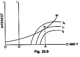
The reason why it slopes upward is, with an increase in income, there are positive effects in liquidity and it increases. With the increase in income, the transactions demand (Lt) and precautionary demand (Lp) for money go up, the demand for idle balances (L_s or L_a) goes down leading to a rise in the rate of interest, this in turn, affects liquidity in a negative manner. But the negative or discouraging effects on liquidity as a result of a rise in the rate of interest are balanced or neutralized by the positive or encouraging effects on liquidity on account of rise in income. Hence, it slopes upward, i.e., Y_L is > 0 and Y_i < 0. Now optimum propensity to consume can be determined in a simple way by combining as shown both parts A and B (Fig. 22.8 and 22.9).

The Fig. 22.9 shows that the slope of iso- Liquidity curve is equal to the slope of iso-investment curve at point P. Positions of O and O’ in the combined diagram are not arbitrary. 00′ shows the difference between total income (OA) and expenditure on consumption (O’A), i.e.,(Y – C = S = I) i.e., it shows the level of investment O’O (OA – AO’ – O’O – I = 00 .

Thus, to each level of investment there belongs a special length of 00′. The optimum propensity to consume is ‘obtained by super-imposing part B (Fig. 22.8) on part A (Fig. 22.7 as shown in Fig. 22.9) and moving it horizontally until the iso-liquidity curve becomes tangent to the iso-investment curve whose index (i.e., level of investment) is equal to the length of OO’. 00′ is the maximum investment, O ‘A and OA are expenditure on consumption and the total income which correspond to it.

Hence, we get general equilibrium and a determinate theory of the rate of interest, where equilibrium level of income, optimum consumption, investment and rate of interest are all simultaneously determined. This is Lange’s approach to general equilibrium analysis by determining the optimum propensity to consume in relation to a rate of interest. It is different from IS—LM curve approach in which the general equilibrium model does not tell us or determine what is the optimum propensity to consume or save. A problem which has been solved by Lange’s model only.