Price Elasticity of Demand Formula | Microeconomics

In this article we will discuss about the formula and equation for calculating the price elasticity of demand explained with the help of examples.

According to the law of demand as the (own) price of a good decreases or increases, the quantity demanded of it would, respectively, increase or decrease. The capacity of demand for a good to increase or decrease in response to a change in its own price is called the price-elasticity of demand.

The coefficient (or measure) of price-elasticity of demand (EP) is obtained by means of the following formula:

[at any (p, q) point on the demand curve for a good]

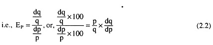
In (2.2) dp is an infinitesimally small change in the price of the good at the initial (p, q) point on its demand curve and dq is the consequential change in quantity demanded of the good. It may be noted here that E_P is defined at a particular point on the demand curve for the good.

The formula (2.1) or (2.2) can be illustrated with the help of a simple example.

Example:

Suppose, when the price of a good is p = Rs 10, the quantity demanded of it is q = 300 units. That is, initially, at the point (p, q) or (10,300) on the demand curve for the good.

Suppose, as p increases from p = 10 to p + dp = 11 (dp = + 1 > 0), q decreases from q = 300 to q + dq = 285 (dq = − 15 < 0). Therefore, here the proportionate and the percentage (p.c.) change in price are = dp/p = +1/10 and dp/p 100% = +10%; also, the proportionate and p.c.

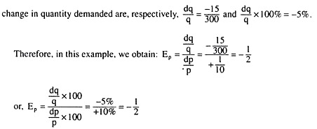
Here, just as an example, take dp = +1, but, actually, in the formula (2.1) or (2.2), dp denotes an infinitesimally small change in p (much smaller than dp = 1).

Remember three things about any coefficient of price-elasticity of demand like E_p = -1/2, that is obtained from above. First, here, it is assumed that coefficient of price-elasticity of demand (E_p) is defined at a point on the demand, curve for the good.

In the above example, [price (p) = Rs 10 and quantity demanded (q) = 300 units] is a particular point on the demand curve. At this point, E_p = -1/2 id obtained. The coefficient of price-elasticity of demand that is obtained at a point on the demand curve is called the point (price-) elasticity of demand, and it is given by the formula (2.1) or (2.2).

Second, owing to the law of demand, i.e., owing to the inverse relation between price and demand; dq ≠ 0 for dp ≠ 0 is obtained, and, as a consequence of this, E_p would be negative (E_p < 0) (since p, q > 0). It should also be remembered that E_p ≥ 0 would be obtained, if there is an exception to the law of demand.

For example, if at any (p > 0, q > 0) point on the demand curve, there is no change in demand (i.e., dq = 0) even when there is a change in price (i.e., dp 0), E_p = 0 [by virtue of (2.2)]is obtained. Again, if at any (p > 0, q > 0) point on the demand curve, price and demand change in the same direction, i.e. as dp ≠ 0, having dq ≠ 0, then E_p > 0.

Therefore, the sign of E_p is very significant. If the law of demand is effective, E_p would be negative (i.e., E_p would be negative owing to the negative relation between price and demand). On the other hand, if there is an exception to the law of demand, E_p would be positive or zero (i.e., E_p would be positive or zero owing to the positive relation or no relation between price and demand).

Third, the value of E_p tells what would be the p.c. change in quantity demanded if price changes by 1 per cent. (Refer to the example given above). When the p.c. change in price is 10, the p.c. change in demand is-5; therefore, when the p.c. change in price is 1, the p.c. change in demand is −5/10 = -1/2 = E_p.

That is, in our example, E_p = −1/2 implies that at the point (p = 10, q = 300) on the demand curve, if the price of the good changes by 1 percent, then its demand would change in the opposite direction (of price change) by 1/2 per cent.