3 Main Forms of Price Discrimination (With Diagram)

The following points will highlight the three main forms of price discrimination.

Price Discrimination Form # 1. First-Degree Price Discrimination:

A firm would wish to charge a different price to different customers.

If it could, it would charge each customer the maximum price that the customer is willing to pay, which is known as reservation price. The practice of charging each customer his reservation price is called first-degree price discrimination.

Let us see how it affects the firm’s profit.

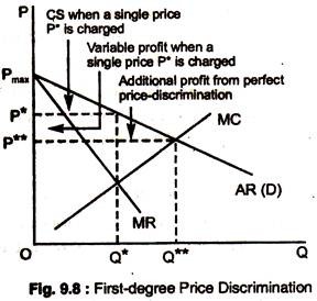
We know the profit the firm earns when it charges the single price P* in Fig. 9.8. To find out, we can add the profit on each incremental unit produced and sold, up to the quantity Q*. This incremental profit is the MR less MC for each unit. In Fig. 9.8, this MR is highest and MC lowest for the first unit.

For each additional unit, MR falls and MC rises, so, the firm produces the total output Q*, where MR = MC. Total profit is simply the sum of the profits each incremental unit produced, and it is given by the area in Fig. 9.8 between the MR and MC curves. Consumer’s surplus, which is the area between the AR curve and the price P* that consumers pay, is shown by a triangle.

What happens if the firm can perfectly discriminate price? Since each consumer is charged exactly what he is willing to pay, the MR curve is no longer relevant to the firm’s output decision. In fact, the incremental revenue earned from each additional unit sold is simply the price paid for that unit, and is, thus, given by the demand curve.

Since price discrimination does not affect the firm’s cost structure, the cost of additional unit is given by the firm’s MC curve. Thus, the profit from producing and selling each incremental unit is the difference between demand and MC. The firm charges each consumer his reservation price, so it is profitable to expand output to Q**.

When a single price P* is charged, the firm’s variable profit is the area between the MR and MC curves. With perfect price discrimination, this profit expands to the area between the demand curve and MC curve. From Fig. 9.8 we can see that total profit is now much larger. Since every customer is being charged the maximum amount he is willing to pay, all consumer’s surplus has been captured by the firm.

In practice, perfect first-degree price discrimination is impossible. First, it is not practical to charge each customer a different price. Second, a firm does not know the reservation price of each customer. Even if the firm could ask each customer how much he would be willing to pay, it would not receive honest answers. After all, it is in the customers’ interest not to give the correct answer!

Sometimes, it can discriminate by charging a few different prices based on estimates of customers’ reservation prices. This often happens when professionals — such as doctors, lawyers, accountants, etc., who know their clients reasonably well — are the firms.

Then, it may be possible to assess the client’s willingness and ability to pay and charge fees accordingly. For example, a doctor may charge a reduced fee to a low-income patient whose ability cum willingness to pay is low, but charge higher fees to upper income patients.

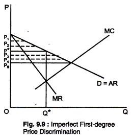
Fig. 9.9 shows this kind of imperfect first- degree price discrimination. If only a single price were charged, it would be P*. Instead, six different prices are charged, the lowest of which, P₅, is just the point where MC intersects the demand curve.

Those customers who would not have been willing to pay a price of P* or greater, are better- off in this situation — they are now enjoying at least some consumer’s surplus. If price discrimination brings enough new customers into the market, consumer welfare can increase, and both consumers and producers are better-off.

Price Discrimination Form # 2. Second-Degree Price Discrimination:

In some markets, each consumer purchases many units of the good over a given period, and consumer’s demand declines with the number of units purchased. For example, water, gas and electricity. Consumers may each purchase a few hundred kilowatt-hours of electricity a month, but their willingness to pay declines with increased consumption.

In this case, a firm can discriminate according to the quantity consumed. This is called second-degree price discrimination, and it operates by charging different prices for different quantities or ‘blocks’ of the same good.

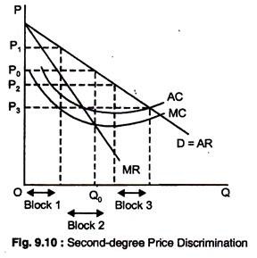
Different prices are charged for different quantities, or “blocks” of the same good. In Fig. 9.10, there are three blocks, with corresponding prices P₁, P₂, P₃. There are also economies of scale, and AC and MC are declining. Second- degree price discrimination can then make consumers better-off by expanding output and lowering cost.

Fig. 9.10 also shows that if a single price were charged, it would be P₀, and the quantity produced would be Q₀, Instead, three different prices are charged, based on the quantities purchased. The blocks are sold at P₁, P₂ and P₃.

Price Discrimination Form # 3. Third-Degree Price Discrimination (P. D.):

A liquor company is practising third-degree price discrimination, and it does so because the practice is profitable. This form of price discrimination divides consumers into two or more groups with separate demand curve for each group.

This is most prevalent form of price discrimination. In each case, some characteristic is used to divide consumers into distinct. groups. For example, for many goods, students and senior citizens are normally willing to pay less on average than the rest of the population and identity can be readily established.

If third-degree price discrimination is feasible, how should the firm decide what price to charge each group? Let us think about this in two steps. First, we know that total output should be divided between the groups of customers, so that the MR_s for all groups are equal.

Otherwise, the firm would not be maximising profit. For example, if there are two groups of customers and the MR for the first group, MR₁, exceeds the MR for the second group, MR₂, the firm could do better by shifting output from the second group to the first.

It would do this by lowering the price to the first group and raising the price to the second group. So whatever the two prices are, they must be such that the MR_s for the different groups are equal.

Second, we know that total output must be such that the MR for each group of consumers is equal to the MC of production (MR = MC). If this was not the case, the firm could increase its profit by raising or lowering total output. For example, suppose the MR_s were the same for each group of consumers, but MR > MC of production.

The firm could increase its profit by expanding the output. It would lower its prices to both groups of customers, so that the MR for each group falls and equals MC.

Algebraically, let us suppose that the price P₁ is charged to the first group of consumers, P₂ the price charged to the second group, and TC(Q_T) the total cost of producing output Q_T = Q₁ + Q₂. Then, total profit is given by: π = P₁Q₁ + P₂Q₂ – TC(Q_T)

The firm should increase its sales to each group of consumers, Q₁ and Q₂, until the incremental profit from the last unit is zero, as given below.

The incremental sales to group one:

dr/dQ₁ = d(P₁Q₁)/dQ₁ – dTC/dQ₁ = 0

Here d(P₁Q₁)/dQ₁ is the incremental revenue from an extra unit of sales to the first group (i.e. MR₁).

The next term, dTC/dQ₁, is the incremental cost of producing this output, i.e. MC.

Thus, we have MR₁ = MC.

Similarly, for the second group, we have: MR₂ = MC.

Bringing them together we get: MR₁ = MR₂ – MC…………. (1)

The relative prices to each group of consumers must be related to their elasticities of demand. We can write MR in terms of the elasticity of demand: MR = P(1 + 1/E_d) and, so, MR₁ = P₁(1 + 1/E₁) and MR₂ = P₂(1 + 1/E₂), where E₁ and E₂ are the elasticities of demand in the first and second markets, respectively.

Now equating MR₁ = MR₂ we get the following relationship for the price P₁/P₂ = (1 + E₂)/(1 + E₁) ………(2) As we can expect, higher price will be charged to consumers with lower elasticity. If the elasticity of demand for consumers in group 1 is -2, and the elasticity of demand for consumers in group 2 is -4, we will have

P₁/P₂= (11/4)/(1-1/2) =  3/4/1/2= 1.5. In other words, Price charged to the first group of consumers should be 1.5 times as high as the price charged to the second group.

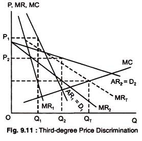
Consumers are divided into two groups, with separate demand curves for each group as in Fig. 9.10. The optimal prices and quantities are such that the MR₁, = MR₂ and equal to the MC. Here, group 1, with demand curve D₁ is charged P₁, and group 2, with more elastic demand curve D₂, is charged the lower price P₂.

The total quantity Q_T is produced where MC = MR and profit is maximised. It may be noted here that Q₁ and Q are chosen so that MR₁ = MR₂ = MC.