Investment Multiplier: Definition, Logic and Assumptions

In this article we will discuss about Investment Multiplier:- 1. Definition of Investment Multiplier 2. Logic of the Investment Multiplier 3. Factors 4. Assumptions 5. Limitations 6. Importance  7. Practical Problems.

Contents:

1. Definition of Investment Multiplier
2. Logic of the Investment Multiplier 
3. Factors Preventing the Investment Multiplier
4. Assumptions of Investment Multiplier
5. Limitations of the Investment Multiplier
6. Importance of the Investment Multiplier
7. Practical Problems with the Simple Multiplier

---

1. Definition of Investment Multiplier:

In his theory of income determina­tion Keynes made the prediction that change in au­tonomous expenditure caused by a shift in any de­sired expenditure function will cause a change in na­tional income. The change in income is greater than or a multiple of the initial change in expenditure. Fol­lowing Keynes we may now consider a change in in­vestment expenditure, which gives rise to the famous multiplier concept.

The multiplier concept developed by Keynes goes by the name investment multiplier (often denoted by the symbol m). It is the number by which the change in investment (∆I) has to be multiplied to find out the resulting change in national income (∆Y).

The income equation in Keynes model is simply expressed as follows:

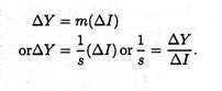
∆Y = m(∆I)

or, m = ∆Y /∆I

Thus the investment multiplier may be defined as the ratio of the change in national income to the ini­tial change in planned investment expenditure that brings it about. Thus, for instance, if a change in in­vestment of Rs. 2000 may cause a change in national income of Rs. 6000, the multiplier is 6000/2000 which is 3.

This value of the multiplier tells us that for every Re. 1 increase in desired investment expenditure, there will be a Rs. 3 increase in equilibrium national in­come. Thus when autonomous investment increases by Rs. 2000 equilibrium national income increase by Rs. 6000.

---

2. Logic of the Investment Multiplier:

What is the logic (or magic) of the multiplier? What is its importance in the theory of income deter­mination? How to determine its value?

In fact, we can answer these three different but in­terrelated questions by adopting any of the following three approaches:

i. An Intuitive Approach:

Keynes first discov­ered that when there is an increase in business firm’s planned investment expenditure on new factors by, say, Rs. 1000 crores per annum, national income would rise by more than Rs. 1000 crores. As soon as the new investment of Rs. 1000 crores is made national income would immediately rise by the same amount. But this is not the whole truth.

This imme­diate and direct rise in income of Rs. 1000 crores (due to a rise in autonomous spending) would be followed by further rise as second (induced) consumption ex­penditure will increase as a result of the increase in national income. But the process of income gener­ation cannot continue indefinitely.

It we ultimately come to a halt when the last increase in consumption spending is not sufficient to generate a fresh income. However, at the end, the total rise in expenditure, and hence in national income, will be more than the rise in autonomous expenditure by the amount of the rise in induced consumption spending.

The above argument may be verified in either of two ways. Since we are dealing with flows of expen­diture, a rise of Rs. 1000 crores in planned investment on new factory construction implies an extra annual expenditure of Rs. 1000 crores on new factories.

Firstly, we can say that the increase in invest­ment expenditure of Rs. 1000 crores per year will in­duce secondary increases in consumption spending. The reason is simple. This extra money will be re­ceived by industries that supply necessary materials for the new factories and those that actually under­take the construction work.

So the initial and direct effect of an increase m autonomous investment of Rs. 1000 crores implies an equivalent increase of employ­ment and income of-factors of production employed in those industries. But the owners of the factors, which find new employment as a result of this new invest­ment, will spend a portion of their new income on consumption goods like food, clothing, shelter, cars, etc. and save the residue.

This increase in consump­tion spending is induced or secondary, not primary. So output has to expand to meet this extra consump­tion demand. The net result is a rise in employment in all of the affected industries.

As and when the owners of factors that are newly employed spend a portion of their incomes (depending on their propensity to consume), employment and output will rise further; more income will be generated and more expenditure induced.

The initial rise in expenditure is an example of a rise in injections. This will lead to an immediate in­crease in income by the same amount. But as income rises, a portion of income will be spent on consump­tion goods and the balance saved. The process of income generation will continue until the additional saving (generated through income increases) is again equated to the additional investment.

In other words, income increase will raise the volume of leakages (in the form of new savings). Income change has to con­tinue until additional saving of Rs. 1000 crores has been generated so as to neutralize the additional in­vestment.

Recall that our initial equilibrium condition of national income is S = I.

If investment increase by ∆I the equality will be converted into an inequality:

S < I + ∆I

or, I + ∆I > S.

But the additional investment will lead to an increase in income (∆Y). This income change will be equal to changes the C and S. So we get ∆Y = ∆C + ∆S. As soon as the additional saving (∆S) is equated to addi­tional investment (∆I), national income equilibrium is restored and we get the following condition:

S + ∆S = I + ∆I.

At this point, desired saving will have risen by as much as the original rise in investment,, and assum­ing that we started from a position of equilibrium, we will return to equilibrium, but at a higher level of income. If, for instance, 1/5 or 20 per cent of income is withdrawn through saving, then the rise in income will come to a halt when income has risen by Rs. 5,000 crores.

When income reaches this higher level, an ex­tra saving of Rs. 1000 crores will have been generated. Moreover since the rise in saving equals the initial rise in investment, the process of income change will ulti­mately stop.

In our example, the increase in national income will stop when it has risen by Rs. 5000 crores. Since ∆Y = m(∆I) or Rs. 5000 crores = m (Rs. 1000 crores), m will be Rs.5000 crores/ Rs. 1000 crores = 5.

In other words, a rise in investment expenditure of Rs. 1000 crores causes a rise in national income of Rs. 5000 crores [So we prove that the multiplier is the ratio of ∆Y to ∆I or the number by which the change in investment has to be multiplied to find out the resulting change in national income.]

ii. A Numerical Approach:

Let us suppose that a hypothetical economy behaved in the following sim­ple way: every time any household receives some ex­tra income it immediately spends 4/5 of it on consump­tion goods (MPC = 4/5) and saves the remaining portion of it. So MPS¹ = 1/5.

Let us now suppose that due to new investment of Rs. 1000 crores there is an increase in injections. As a result national income raises by Rs. 1000 crores im­mediately. But this is not the whole truth. The owners of factors directly and indirectly engaged in produc­ing the investment (capital) goods will utilise Rs. 800 crores. each year to buy consumption goods and save the remainder (i.e., Rs. 200 crores).

In an interde­pendent economy one man’s expenditure is another man’s income. Now those who receive this Rs. 800 crores, in turn, spend an extra Rs. 640 crores a year (4/5 of Rs. 800 crores). Thus there is a further addition to aggregate expenditure. The process will continue for some time and at any stage of the process each successive set of recipients of new income spend 4/5 of their new income and save the rest.

Such extra expenditure, in its turn, creates fur­ther (new) income and a portion of this extra income is again spent on consumption good (and the balance saved). The process is described in the above table. Table 35.1 carries the whole process in 10 rounds. We observe that the sum of all of this new expenditure is approximately Rs. 5000 crores.

This final total is five times the initial new injection of Rs 1000 crores of au­tonomous expenditure (investment). Thus the value of the multiplier is 5, i.e., Rs. 5000 crores = 5 x Rs. 1000 crores.

This value is derived on the basis of the assump­tions about consumption and saving. According to Paul Samuelson and W.B. Nordhaus, “an increase in income will increase GNP by an amount greater than itself. Investment spending is high-powered spend­ing”.

The amplified effect of investment on output is called the multiplier. The term ‘multiplier’ is used to refer to the numerical coefficient showing the size of the increase in output resulting from each unit in­crease in autonomous investment.

iii. A Graphical Approach:

The multiplier may also be illustrated graphical. Fig. 35.9 illustrates the multiplier concept graphically. It is a graphical representation of the results of Table 35.1. The white bar in each period shows how much income has been generated in the previous period.

The shaded bar shows the increase in the amount per period, which is 4/5 of the income of the previ­ous period. The total height of the two parts of each bar shows total income in the relevant period. Total income shown by the last bar is sum of primary in­vestment and secondary consumption.

According to Samuelson, “an endless chain of secondary consump­tion spending is set in motion by a primary investment spending. But, although it is an endless chain, it is a dwindling chain. And it eventually adds to a finite amount”.

In Fig. 35.10 income is initially assumed to be in equilibrium at Rs. 80,000 crores. Now suppose autonomous investment increase by Rs. 1000 crores from Rs. 30,000 crores to Rs. 31,000 crores. This may occur if business firms increase their spending on new factories. This is shown by an upward shift of the in­vestment curve from I to I’.

Consequently national income increases by Rs. 5000 crores—from Rs. 80,000 crores to Rs. 85,000 crores .This increase which is shown by ∆Y in Fig. 35.10 is larger than the in­crease in investment which is shown by ∆I which caused the increase in income.

The ratio of the two absolute changes is the mul­tiplier, m or, we have

m = ∆Y/∆I = Rs. 5000 crores/Rs. 1000 crores = 5.

In the words of J. Breadshaw, “The multiplier principle is that a change in the level of injections (or withdraw is) bring about a relatively greater change in the level of national income.” This again tells us that for every Re. 1 increase in autonomous investment expenditure, equilibrium national income increased by Rs. 5.

Thus the multiplier can be defined as the ratio of the (absolute) change in equilibrium income to the initiating change in autonomous investment that brought it about.

We may now consider Fig. 35.11. We see that the size of change in income brought about by a shift in the investment schedule from I to I’ differs according to the slope of the saving curve. Here we present three saving curves with different slopes.

The slopes of S, S’ and S” are 0.40, 0.20, 0.133, respectively. The respective change in equilibrium income in response to shift of the investment schedules from Rs. 31,000 crores to Rs. 31,000 crores are ∆Y₀ = Rs. 2500 crores, ∆Y₂ = Rs. 5000 crores and ∆Y₃ = Rs. 7500 crores.

The numerical values of the multiplier in these three cases are 2.5, 5 and 7.5, respectively. This shows that the flatter the saving schedule, the larger the value of the multiplier.

It is because the slope of the saying schedule is the MPS and the reciprocal of the slope of the saving schedule gives us the value of the mul­tiplier. Therefore, the flatter the saving schedule, the larger must be the increase in income, before saving rises to equal the new level of investment.

The Relation between the Propensity to Consume and the Investment Multiplier:

The multiplier is the reciprocal of MPS. We know that MPS = 1 – MPC. Therefore there is a close relation between MPS and the investment multiplier.

We can express the multiplier as follows:

m = 1/MPS = 1/1-MPC

If we denote MPS by s and MPC by b we can ex­press the multiplier as: m = 1/s = 1/1-b. The example given in Table 35.1 brings into focus two points:

(1) The larger the MPC the higher the numerical value of the multiplier will be.

(2) For the concept of the multiplier to be meaningful b must lie in-between zero and one. Or, in other words, it must be greater than zero but less than one.

In fact, by putting different values of b we get dif­ferent values of s since b + s = 1. And corresponding to each value of s, we have a specific value of ∆Y for a fixed level of exogenous investment. And the same level of investment gives us different levels of income. Only where b = 0 and s = 1, there is no responding on consumption and m = 1.

The point that the multiplier is the reciprocal of MPS may be clarified further by referring to Fig. 35.10. The figure illustrates that when the economy has moved from its original to its new equilibrium point, the change in saving has to be equal to the change in investment, i.e., ∆I = ∆S. Thus we can express the multiplier as m = ∆Y/∆S.

The slope of the saving curve is ∆S/∆Y. Thus, the multiplier, ∆Y/∆S, is the reciprocal of the slope of the saving function. Thus if we know the value of the MPS we can predict the effect of a change in investment upon na­tional income.

The effect will be the change in invest­ment multiplied by m or we can write:

Problem 1:

Suppose I = Rs. 70; C – Rs. 60 + 0.80 Y. (a) Find the equilibrium level of income, (b) Find the equilibrium level of income when there is a Rs. 10 increase in autonomous planned investment (planned investment increases from Rs. 70 to Rs. 80). (c) Establish the multiplier effect of the Rs. 10 increase in autonomous spending.

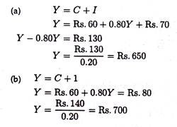
(c) The equilibrium level of income increases by Rs. 50 (from Rs. 650 to Rs. 700) as a result of a Rs. 10 increase in investment. There is a multiplier effect of 5 (that is, ∆Y/∆I = Rs. 50/ Rs. 10 = 5) as a result of the increase in autonomous investment.

Problem 3:

Derive the multiplier when the MPC is 0.90, 0.80, 0.75 and 0.50. (b) What is the relationship between the marginal propensity to con­sume and the value of the multiplier? (c) Use the multiplier values found in (a) to establish what effect a Rs. 20 decrease in autonomous spending has upon equilibrium income.

Sol:

(a) The multiplier m equals 1/(1-b), thus, m is 10 when the MPC is 0.90; 5 when MPC is 0.80; 4 when MPC is 0.75; and 2 when MPC is 0.50.

(b) There is a multiplier effect because consump­tion spending is related to the level of disposable in­come. Any change in income induces a change in aggregate consumption, with the magnitude of the change dependent on the value of the marginal propensity to consume. Thus, the value of the mul­tiplier is directly related to the value of the marginal propensity to consume.

(c) The decline in income equals ∆Ī(m). The de­crease in equilibrium income is Rs. 200, Rs. 100, Rs. 80 and Rs. 40 for the four values of MPC. respec­tively.

Problem 4:

If investment falls Rs. 20 and the marginal propensity to consume is 0.60, what are (a) the change in the equilibrium level of income, (b) the change in autonomous spending and (c) the induced Change in consumption spending?

Sol:

(a) The change in the equilibrium level of income equals m∆Ī. Since m = 2.5, ∆Y = – Rs. 50.

(b) The Rs. 20 decline in investment is the change in autonomous spending.

(c) The induced change in spending is the dif­ference between the change in the level of income and the change in autonomous spending. That is ∆Y – ∆Ī = ∆C. Induced spending falls by Rs. 30.

Temporary and Permanent Change in the Equi­librium level of National Income: [Optional Read­ing]

J. Beardshaw pointed out that for the change in the equilibrium level of national income to be perma­nent, it is necessary that the increase in investment is also of a permanent nature. In our previous example, the Rs. 1000 crores of one-for-all investment would lead to once-for-all increase in national income of Rs. 5000 crores and then the equilibrium would return to its previous level.

On the other hand, if there was a continuous injection of investment of Rs. 1000 crores in each time period then there would be a permanent increase in the equilibrium level of national income of Rs. 5000 crores as is illustrated in Fig. 35.12.

 

---

3. Factors Preventing the Investment Multiplier:

Various factors prevent the multiplier working out as precisely as has been suggested by Keynes in his General Theory.

The following factors deserve mention in this context:

i. Personal Disposal Income:

Keynes stated that the size of the multiplier is determined by the MPC. However, the MPC is calculated from PDI, but be­fore extra spending in the economy can become PDI, it is first received by firms, who may retain part of it for reserves or for depreciation and will also pay part of it to the government in tax. For these reasons the value of the multiplier may get reduced.

ii. Type of Investment:

Different types of invest­ment will have different multiplier effects. For exam­ple, extra defence spending is likely have a different effect from spending on house building because the MPCs of the recipients will vary widely. Moreover certain categories of investment spending will create a more favourable economic climate, thus bringing about more investment.

iii. Time Lags:

The time taken for the multiplier process to work itself out through the various ’rounds’ of spending may vary.

iv. Other Multipliers:

The theory of the multiplier was developed in the midst of the depression of the 1930s by Richard (later Lord) Kahn. However, he wrote about an em­ployment multiplier in 1931. He observed the millions of unemployed and suggested that if more men are employed they would spend their wages.

This, in its turn, would create new jobs for other men, and so on. J.M. Keynes developed in 1936 the investment multiplier. He shifted emphasis from job to aggregate spending.

At a later stage various other multipliers, such as the Government expenditure multiplier, bal­anced budget multiplier and foreign trade multiplier have been incorporated into the theory of income de­termination.

Problem 5:

An imaginary economy is in equilibrium with no foreign trade or government activity. The aver­age propensity to consume and the marginal propensity to consume are both 8/10, the actual level of consumption expenditure being Rs. 16,000 in each year.

(a) Explain the italicized phrases.

(b) What is the level of investment expenditure each year?

(c) What is the value of the multiplier? Suppose that with investment expenditure unchanged both average and marginal pro­pensities to consume drop to 3/4.

(d) What will be the new equilibrium level of national income?

(e) Explain briefly the effects on the equilibrium of this simple system, by introducing foreign trade and government activity.

Sol.

(a) The propensity to consume represents that proportion of income which is spent. The propor­tion of income spent is not constant however, at very low levels of income people will even draw on their savings and spending on consumption will actually exceed income.

At high levels of income the propor­tion of income spent falls. The average propensity to consume is the mathematical average of these. The marginal propensity to consume relates to the pro­portion of additional income that people spend.

(b) If consumption expenditure is Rs. 16,000 and this represents an MPC of 8/10 then Rs. 16,000 = 8/10 of investment injected. Hence the investment injected = Rs. 20,000. But 2/10 (i.e., Rs. 4000) is investment expenditure.

(c) As MPC = 8/10 then MPS = 2/10 and the multiplier must be the reciprocal of the latter i.e.,10/2 i.e., 5.

(d)If MPC = 3/4 then MPS = 1/4. But this 1/4 rep­resents Rs. 4000 since investment expenditure (i.e., amount saved) is unchanged. Hence the new equilib­rium level of national income must be Rs. 16,000 (i.e., 4x Rs. 4000).

(e) Foreign trade would result in importing of goods and government activity would result in taxa­tion. These represent leakages in the system and the value of the multiplier would fall and the increase in national income resulting from an injection of invest­ment will be lower than if there were no international trade or government activity.

However, both inter­national trade and government activity have reverse sides in the form of exports and government expen­diture which represent further injections.

---

4. Assumptions of Investment Multiplier:

Keynes’ multiplier principle is based on the fol­lowing assumptions:

i. Autonomous Investment:

It comes into operation for any autonomous change in spending, viz., investment, government spending, export and consumption.

ii. Lump-Sum Taxes:

Taxes are assumed to be lump sum only. If a portion of increased income is taxes away at every stage of income generation the multiplier effect will be smaller.

iii. Availability of Consumption Goods:

The process of income-propagation is largely conditioned by a steady flow of mass consumption goods.

iv. Continuity of Investment:

For the realisation of the full effect of the multiplier it is absolutely essen­tial that the various increments in investment are repeated at periodic intervals.

v. Positive Net Investment:

For realizing the full value of the multiplier it is not enough for gross in­vestment to be positive. Gross investment to the extent of depreciation always take place in any economy. But net investment or net addition to society’s stock of capital has to be positive.

vi. Stability of MPC:

For the concept of the multiplier to be meaningful it is also necessary to argue that there is no change in MPC at frequent inter­vals, i.e., at least during the process of income- generation.

vii. Closed Economy:

We assume a closed economy having no trading relation with the rest of the world.

viii. No Time Lag Between Successive Expenditures on Con­sumption Goods:

It is argued the income changes are immediately reflected in consumption changes. There is no lag between receipt of in­come and expenditure on consumption.

ix. Unemployed Resources:

Finally, Keynes argued that the multiplier principle becomes effective only when there are unemployed resource in the econ­omy. In other words, there must exist involun­tary idleness of resources including manpower.

---

5. Limitations of the Investment Multiplier:

The concept of the multiplier to be meaningful M PC must be greater than zero but less than one. This is so because there are various leakages from the circular flow of income. Due to these leakages the process of income genera­tion slows down.

If MPC = 3/5 or 60 per cent the implication is that 2/5 or 40 per cent of the new income leaks out or is withdrawn from the circular flow of income. So the remaining 60 per cent is spent on con­sumption goods.

The most important leakages from the circular flow of income are the following:

i. Saving:

It is the most important leakage. If MPC = 1 and MPS = 0 the numerical value of the multiplier would approach infinity. This means that if the entire new income created by an act of in­vestment at each stage of the income generation pro­cess were spent by the people on buying consumer goods, then even a once-for-all increase in investment would go on creating extra income until the economy reached the stage of full employment. But MPC is rarely equal to 1.

In practice, people hardly spend their entire income on consumption goods. They save a certain portion. The portion they save (i.e., do not spent) disappears from the circular flow, thus reduc­ing the value of the multiplier. Thus the stronger the MPS of the people, the smaller will be the value of the investment multiplier.

ii. Debt Repayment:

James Duesenberry has pointed out people do not spend their entire extra income on consumption good. They use a part of it to repay their past debt. As a result, the value of the multiplier gets reduced.

iii. Accumulation of Idle Cash Balances:

People often save money by keeping idle cash balances in banks. This idle money does not come into circulation and is unlikely to lead to an increase in consumption spend­ing.

iv. Stock Exchange Transactions:

It is often observed that a major portion of the new income gen­erated in the economy is utilised to buy old bonds and securities from others. Most people sell these long-term credit instruments when in distress and in­cur capital losses. So such transactions are unlikely to raise society’s total consumption appreciably.

v. Imports:

No country in the world is self- sufficient. Therefore, a country has to spend some money on imports. However imports do not add to domestic expenditure and is unlikely to have any income and employment effect.

To the extent we spend a certain portion of our new income on im­ported goods, money leaks out of the country. In other words, the value of imports peters out of the income-stream, thus limiting the value of the multi­plier.

vi. Price Inflation:

During inflation money in­come may rise but real income falls. Thus real con­sumption spending (which determines the value of the multiplier) will fall. In other words, a major por­tion of increased money income will be neutralised by price inflation, instead of stimulating consumption and creating jobs and incomes in the process.

vii. Taxes:

If the government taxes away a certain portion of the extra income generated in the economy the value of the multiplier will fall. So like savings, taxes also act as a leakage from the circular flow. Taxes are contractionary in their effects in-as-much as they reduce real consumption spending by reducing dis­posable income.

viii. Corporate Savings:

Moreover companies do not always distribute their entire net profit (gross prof­its less corporation tax) as dividend. They retain a certain portion for expansion and diversification. To the extent they follow the policy of saving a certain portion of their net profits the consumption spend­ing of shareholders fails to increase correspondingly. Therefore the value of the multiplier will be less than otherwise.

Conclusion:

There is no denying the fact that due to such leakages the process of income genera­tion slows down after some time. If such leakages in income stream did not exist, the process of income generation would come to a halt only when a state of full employment was reached. In fact, the process of income propagation could go on until there was the end of full employment or the beginning of inflation.

According to Keynes, full employment is the econ­omy’s inflation threshold. True inflation occurs only when the economy has just moved passed the stage of full employment. To the extent to which the leak­ages could be identified and their severity reduced the value of the multiplier would increase and the process of income generation would become faster than before.

The Reverse Investment Multiplier:

The multiplier process also works for a fall in investment with a subsequent fall in income. If MPC = 4/5 and investment falls by Rs. 1000 crores national income will fall by Rs. 5000 crores. This will reduce the level of saving by Rs. 1000 crores because MPS = 1/5. So the new level of equilibrium will be reached when S = I = Rs. 4000 crore or where the desire to save and the desire to invest are once again equal.

---

6. Importance of the Investment Multiplier:

Keynes’ theory of investment multiplier is con­sidered to be an important and permanent contribu­tion to economic theory. However, it is not only a the­oretical concept showing the magnified effect on na­tional income of a small change in autonomous invest­ment. The concept has highlighted the importance of investment as the major dynamic element in economy. But it has practical relevance, too.

It can be used to make a strong case for public investment, particularly in a period of deep depression and widespread unem­ployment. It is because a small increase in public ex­penditure at such a time may lead to a large increase in income, output and employment. The concept is also useful to governments in formulating an appropriate employment policy during depression.

The concept has brought into focus the important point that em­ployment is directly created by investment. It has also clearly revealed that income is generated throughout the economy due to secondary consumption spend­ing (which is induced by an initial or primary act of investment).

Moreover, a background knowledge of the multiplier is of paramount importance not only in analysing business cycle movements but in formulat­ing an appropriate counter-cyclical fiscal policy which seeks to achieve economic stability.

However, its usefulness as an accurate means of economic prediction of future developments depends upon the reliability of the assumptions which must be made. Specifically we must assume that the aggregate MPS is both measurable and constant during any likely future changes in income.

This, of course, is an unrealistic assumption. A change in the pattern of in­come distribution, for instance, will alter the value of MPS and thus the value of the multiplier in the pro­cess.

But, if we accept this fundamental assumption two useful applications are possible:

1. The multiplier can be used by governments and by businessmen to forecast the overall effect of a public expenditure programme. For example, if it is known that Rs. 500 crores will be spent in building new roads in Calcutta and it is cal­culated that the aggregate MPC is 3/4 then total income will rise by Rs. 2000 crore and total con­sumption by Rs. 1500crore.

The government can now assess its effect on the economy as a whole and especially on the level of employment. A company which produces consumer goods may be able to forecast how the overall rise in demand will affect the demand for its production.

2. The level of investment is a function of the level of income. Therefore the government can use the multiplier to determine the policy needed to achieve full employment. For example, if India’s national income is Rs. 50,000 crore and it is esti­mated that a level of Rs. 60,000 crore is desirable to overcome unemployment, the government can estimate how much additional investment is re­quired to reach the goal.

If the MPC = 3/4, the calculation is

Y = m (∆I)

or, Rs. 10,000 crore = 4x ∆I

or, ∆I = Rs. 10,000 crore/4 = Rs. 2500 crore.

Thus an increase in investment of Rs. 2500 crores is desirable. This amount is known as the defla­tionary gap, that is, the initial increase in aggregate demand which is necessary to eliminate unem­ployment.

Alternatively, if the economy is moving towards a level of national income of 65,000 crore, and the gov­ernment fears that this will cause an undesirable rate of inflation it may take steps to reduce aggregate de­mand. If it wishes to stabilize the national income at Rs. 60,000 crore, it can calculate by how much invest­ment must be reduced of MPC = 3/4.

-Rs. 5.000 = 4∆I

or, ∆I = 1250 crore

This required fall in investment of Rs. 1250 crore is known as the inflationary gap.

It shows the amount by which aggregate demand must be reduced initially to prevent any excess of de­mand over supply that will cause prices to rise.

The government generally does not wish to influ­ence the level of investment. So the same effect may be achieved by a similar change in the level of planned consumption or the level of government expenditure.

---

7. Practical Problems with the Simple Multiplier:

These are certain practical problems associated with the multiplier.

The following are the most im­portant in this context:

i. The Calculation of the Aggregate MPC:

It is dif­ficult to calculate aggregate MPC. It can be cal­culated for changes in the level of income in the past. But projection of the aggregate consump­tion function based on past data is unrealistic be­cause the behaviour of the people may change.

ii. A Change in the Distribution of Income:

In re­ality any multiplier increase in income hardly gets distributed evenly throughout the popula­tion. So a redistribution of income is likely. This may affect the aggregate MPC.

Thus if a new in­vestment project takes place in a village, where, because incomes in general have been low for some time, the average MPC is high, the mul­tiplier effect will be greater than if the same in­vestment is made in Calcutta where the MPS is high.

iii. An Induced Change in Consumption:

A multi­plier increase in income may create expectation of further rises and so cause people to spend more out of a given income and will set off further mul­tiplier effects

iv. Induced Changes in Investment:

If we consider induced investment also, income change will be greater. A multiplier effect which increases con­sumption and brightens investment prospects will induce increases in investment.

This, in its in turn, will lead to further multiplier process. That is, if investment like consumption depends on income or its change, the multiplier effect will be stronger. From this proposition Sir John Hicks developed the concept of super-multiplier.

v. An Output Lag:

If there is an output lag, i.e., if producers do not immediately increase output to meet an increase in total demand and allow their stocks of goods to run down, the multiplier effect will be partly lost. The same thing happens if there is consumption lag, i.e., if households who receive an increase in their income take time to adjust their consumption habits.

vi. Business Saving:

Finally, if companies do not distribute the major portion of their profits to shareholders in the form of dividends and in­crease their reserves of undistributed profits the aggregate MPS will rise and the size of the mul­tiplier is reduced.

Conversely, “when incomes are falling, companies may sell down their re­sources and pay dividends in excess of current profits. This increases disposable income and so weaken the multiplier fall in total incomes.”

---