Dynamic Multiplier Action in Net Investment of an Industry

Read this article to learn about the dynamic multiplier action in net investment of an industry.

In the actual world adjustment as a result of change in net investment takes time.

Therefore, to get a more complete picture of the events connected with a change in net investment, we have to follow the path of movement from one equilibrium situation to another equilibrium situation.

An enquiry into the process of movement requires the treatment of multiplier problem in terms of dynamic analysis. In other words, the analysis of a single investment shock can be easily extended to cover the analysis of effects over time of a permanent change in net investment. A permanent increase in net investment is a continuous series of investment shocks of equal size.

Let the initial and original equilibrium be disturbed by a permanent increase in net investment of 100 per period of time. The level of investment now exceeds the original level of 100, not only in period 1 but in all the following periods. In each period an investment of 100 now takes place. We simply add the effects over time of the individual investment shocks to obtain the total effect of the rise in the level of net investment. Let us further assume that all transactors have a MPC of ½ and that they react to a change in income in any one period by changing consumption expenditure only in the following period.

On these assumptions, the process resulting from a permanent increase in net investment of 100 per period is as follows:

In period 1 income rises by 100. In period 2 this increase in income leads to an increase in consumption of 50 and thus to a rise in income above the original level of 50. But in period 2 there is again additional investment shock of 100, and thus a further increase in income of 100, so that the total increase in income (over the original level) in period 2 is 150.

In period 3 the rise in income is 175, including an additional investment of 100 in period 3, but increased consumption expenditure is 50 (resulting from the increase in income due to increase in investment in period 2) and of 25 increased consumption expenditure (resulting from the increase in income due to the increase in consumption expenditure in period 2) and so on, as shown in the table given above.

The arrow pointing from the investment of one period shows the effect of a single investment shock. The horizontal line for any one period contains the components of the increase in income during that period, and shows from which investment shock the individual component derive.

With a MPC of ½, the increase in income in the individual periods is shown by the following expressions:

1st period: 100

2nd period: 100 + ½ .100

3rd period: 100 + ½ .100 + (½)² .100

4th period: 100 + ½100 + (½)² 100 + (½)³ 100.

nth period: 100 + ½ . 100 + (½)² 100 + (½)³ . 100+….+(½)^n-1.100

The increase in income in the nth period represents a(∆Y) geometric series of n terms with a ratio ½.

According to a formula for the sum of a finite geometric series the increase in income (∆Y)_n is given by :

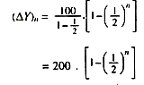
Since (½)ⁿ tends towards zero as n increases. (∆Y_n) increases with n and approaches 200. Thus, we have

The table given below shows the working of the dynamic multiplier and the equilibrium process between S and I:

The table shows economy as starting out from a low position of equilibrium, where income in period 0 equals consumption conditioned by previous income plus current investment, or 100 = 80 + 20, and where S = 1. As a sudden increase of investment with an increment of 10, income also increases by 10 to increase total income to 110. But consumption does not immediately react to the increment of income and remains at 80. Investment has gone up to 30, and yet intended savings remain at 20.

Thus, the difference between investment and intended savings equals unexpected extra income, or ∆C + ∆I – ∆Y (0 + 10 = 10). So ends period 1 and period 2 begins. In period 2 consumption increases by 5 which is half of previous extra income 10. Intended savings, thus increase by 5, with an increase in income by the increment of consumption or, we can say, by the difference between investment and savings.

Total income earned or produced in period 2 equals 115 which is 5 over preceding period. As the unchanged investment still exceeds intended savings by 5 in period 2, this is the amount by which income in the next period will expand, and so it will go on. In period n, extra investment of 10 reaches its limit, for it is no longer capable of generating additional consumption and savings on a 50 per cent basis. Total savings have increased enough to cancel out the extra investment plus the original investment, or 30 = 30. The multiplier has caused total income to reach the asymptote, and consumption and savings with it.

It should be noticed that total income in the final stationary level is exactly 20 more than at the initial level, according to ∆Y= K. ∆I yet it has taken time for extra investment of 10 to lift total income by an amount equal to K times ∆I. Thus, by showing income behaviour through discrete q stages the dynamic multiplier analysis based on difference equations makes an important contribution to the theory of economic fluctuations.

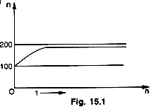
The figure 15.2 and the table given above show the increase in (∆Y)_n as n increases. With a MPC of 1/2 the final effect of a permanent increase in net investment of 100 is a permanent rise in national income of 200. The curve in the figure 30 shows the path by which this increase is finally attained. As can be seen, the final effect of the multiplier process is achieved only after an infinite number of periods ; in actual practice, however, the new higher equilibrium level of income is reached after a few periods (in our example after five periods). This dynamic process of income generation is shown diagrammatically also in the figure given below.

We assume that consumption depends on the income of the proceeding period, C – C_t = a Y_t-1 where a is the marginal propensity to consume and also that investment is a function of income and an autonomous constant I = I_t = I. In the above diagram, consumption, investment and savings are measured along the vertical axis and income is measured along the horizontal axis—all magnitudes being in real terms.

Thus, C curve relates consumption to the income of the preceding period and it has a constant slope of 0.5. The original investment schedule is a vertical distance between the C curve and the C_+ I curve, while the new investment schedule is that between the C curve and the C + I + ∆I curve, which gives a constant level of investment equal to ∆I. Savings out of previous income are measured by the vertical distance between the 45° line and the C curve. The system is initially settled at equilibrium point E₀, where savings and investment are equal (E₀C₁ = E₀C₁). This is our starting point.

In period 0, before the change, consumption is C₁Y₀ and income OY₀ or E₀Y₀, thus leaving E₀C₁ both as saving and investment. Now investment increases by ∆I from period 0 to period 1 and stays at this level. What is the effect of this? Consumption remains unchanged because consumers have not yet had an opportunity to adjust themselves to change. Similarly, intended savings remain unchanged. This means that investment exceeds intended savings by an amount equal to the increment of investment, or by Y₁E₀. This excess of investment over intended savings for period 1 (equal to actual savings for period 0) account for the unexpected increment of income from period 0 to period 1.

In period 1 there is an equal horizontal change. Y₁E₁ (= Y₀Y₁), for the vertical change of Y₁Eo- In other words, income increases over OY₀ by the amount of excess investment in period 1 after the injection of ∆I . The total income received in period 1 is therefore OY₁ (= OY₀_+ Y_oY₁). What would happen to saving investment relation in this period? Investment is again I + ∆I or Y₂C₂ and savings corresponding to previous income OY₀ are E₁C₂, thus making intended savings fall short of investment by Y₂E₁ (=Y₂C₂ – E₁C₂). This excess investment is what causes income to increase from period / to the next, that is, by Y₁Y₂ (= Y₂E₂ = Y₂E₁).

Though consumption increases from C₁Y₀ to C₂Y₁ corresponding to the increased total income of OY₁, this extra consumption amounts to half of extra income Y₀Y₁. Similarly, savings increase by half of extra income Y₀Y₁. This explains why intended savings in period 1 fall short of investment.

As such income expands by an amount equal to the above excess of investment over intended savings, or by Y₂E₁, which amount is equal to the horizontal change of Y₂E₂. It is thus that period 2 is ushered in and total income received is OY₂. But investment in this period still exceeds saving by Y₃E₂ (= Y₃C₃ – E₂C₃), since intended savings corresponding to previous income OY₁ amount to E₂C₃ which amount is Y₃,E₂ short of a total investment of Y₃C₃ (constant I + ∆I ). This excess of investment over intended saving in period 2 leads to an increase in income from period 2 to period 3 ; and so on.

It may be noted that the gap between intended saving and intended investment (the vertical distance between the C + I + ∆I curve and the 45° line) becomes smaller and the increment of income which it produces, until the gap is completely wiped out. The constant stream of new investment has developed its full effect and aggregate income has reached the stationary higher level of Y_n in the nth period. The system has become stable at the new and higher equilibrium point E_n.

Income has reached there via E₀, Y₁, Y₂, E₂,…, E_n. The multiplier has done its job, for it has caused income to expand to cause intended savings to expand up to the new level of investment ; that is, where S_n=I_n. Thus, in the nth period the savings gap (the vertical distance between the 45° vertical line and the C curve at Y_n) exactly equals the sum of old investment plus new investment (the vertical distance between the C + I + ∆I curve and the C curve at (Y_n).

This attempt towards the generalization of the multiplier is very light but it does do something to put the theory into the form which we need for further investigations. There is hardly any doubt that in actual practice the response of consumption to changes in income is lagged; “indeed” says Hicks, “the multiplier theory cannot be stated in a compelling form unless the lags are recognized”.

Of the two classical formulations, it is the lagged version of Mr. Kahn which is more easily intelligible; the lag-less version of Keynes, in spite of its technical simplicity, is not acceptable’. If there is an economically significant time lag between an initial investment expenditure and its reappearance as income, difference equations expressing lagged consumption and investment must replace static equations in order that the discrete steps involved in the multiplier process may be traced.

A simple dynamic system involving a consumption lag but no investment lag is as follows :

where C_t is consumption at time t, a the marginal propensity to consume, Y_t-1 previous income, Y₀ initial income, C₀ initial consumption, I_t investment at a time t, and I constant autonomous investment. The essential point to notice about the general multiplier equation (iv) is that consumption is lagged, i.e., dependent on the income of the proceeding period over and above some arbitrary initial income.

Qualifications:

(i) Allowance has to be made for the possibility that the MPC may not remain constant as income increases through the multiplier action.

(ii) However high the MPC may be, output and employment will stop growing, once full employment has been reached. Beyond that level a further increase of investment would merely increase general prices.

(iii) The assumption of a given increase of investment though useful may have to be dropped in order to allow for the possibility that the multiplied income may, in turn, induce fluctua­tions in investment.

(iv) Allowance must be made for the possibility that a part of the magnified income may leak out to the benefit of employment elsewhere, as far as an open system with foreign trade relations is concerned.