Market Mechanism in Economics: Examples and Graphs

In this article we will discuss about:- 1. What is Market Mechanism 2. Efficiency under Market Mechanism 3. Examples 4. Graphs.

What is Market Mechanism:

Market mechanism is often interpreted as a ‘free’ market system. For a layman ‘free’ means that when you go to a market, there is no re­striction – you can buy as much as you want OR sell any amount OR choose to do nothing.

You are free to take decisions regarding buying and selling. Adam Smith used this freedom to formulate the notion of an ‘invisible’ hand.

‘Invisible hand’ refers to the individual actions/decisions of economic agents that lead to maximum welfare for the economy. It is as if an in­visible force strings together decisions, taken in self-interest by different persons, to give us a result which is the best for all persons considered together.

These decisions operate in terms of demand and supply for a good, which are collectively referred to as the market mechanism. Thus, the market mechanism ensures that the benefits/welfare for the whole group of economic agents is a maximum. This only requires that each agent operates on the basis of self-interest and decides what is best for her alone, assuming there is freedom given to each of them.

Free market is also associated with a capitalist economy, as opposed to socialist economy where markets follow plans made by the government. This reduces the ‘freedom’ of the market mechanism, though a ‘market’ may still exist. The ‘freedom’ given to market mechanism is therefore the crucial distinction between capitalism and socialism.

For example in India, we have a free market for medicines/drugs. Anyone can buy a drug with a prescription or any out-the-counter drug that needs no prescription. This implies buyers and sellers are ‘free’ to buy and sell any quantity at any price; it is a free market. But the National Pharma Pricing Authority (NPPA) has put limits on the prices of some selected drugs called essential drugs. This means that producers/pharma com­panies cannot charge any price they want. This restricts the ‘freedom’ of sellers, and is an example of restriction on the market.

As the above example makes clear, the market mechanism refers to the forces of demand and supply. These forces take the form of buyers and sellers in the market. Economists show that if left ‘free’ these forces use the self-interest of sellers and buyers to reach a point where welfare for all is maximized.

The ‘mechanism’ refers to the fact that economic agents (buyers and sellers) act in self-interest without any force on them and without any explicit coordination between themselves to maximize their own welfare. In this process the sum total of welfare/gain for all economic agents in an economy is maximized. As compared to any other mechanism (like planning by State in a socialist system) the welfare to society as a whole is maximum in market mechanism.

Efficiency under Market Mechanism:

In everyday use, efficiency means to work in the best possible way, or in a ‘smart’ way that reduces time taken for any work and makes sure that efforts are not wasted. In Economics ‘efficiency’ is defined in more clear ways. Alfred Pareto was the first economist to define efficiency, and accordingly we define optimality in terms of Pareto efficient states. According to Pareto, “a Pareto efficient state of affairs is when no one can be made better off without making someone worse off”.

Take an example:

Original state-Suppose Vineet earns Rs.10000 per month and Radhika earns Rs.15000 per month working for their manager Mr. Diwan. Total income will be Rs.25000. Welfare will be measured in terms of salaries of both workers and other office costs for Mr. Diwan (electricity, water, rent are some costs incurred in a typical office). Assume that costs equal Rs.5000 for simplicity. Let us consider three options to this original state of affairs. Welfare equals the sum of salaries and other costs = Rs.30000

State 1:

Let both employees argue for higher salary with Mr. Diwan, who refuses to do so as his costs will rise. Instead he offers to change the distribution; he offers Rs.12000 to Vineet and Rs.13000 to Radhika. Now this proposed state makes Vineet better off, but Radhika worse off and Mr. Diwan do not change his costs.

Total welfare remains at Rs.30000. This proposed income change is Not a Pareto improvement over the original income distribution, because one person has been made better off at the cost of someone else being worse off.

State 2:

Instead if Mr. Diwan increases salary for both by an equal amount (however small, say Rs. 500), while reducing his costs on other inputs by Rs. 1000, then it is a Pareto improvement. This is because both will be better off, with none of them worse off.

State 3:

Another option is that Mr. Diwan increases salary for Vineet by Rs. 600 and by Rs. 400 for Radhika. If he does this by reducing his other costs by Rs. 1000, so that Mr. Diwan does not face higher total costs, then this is also a Pareto improvement as both have gained, while Mr. Diwan has not lost as well.

As long as we can make Pareto improvements as outlined in options 2 and 3, we are not efficient. When no Pareto improvements are possible, we have reached an efficient state. In other words, a Pareto efficient state is achieved when there are no Pareto improvements are possible.

Efficiency is also sometimes used interchangeably with Pareto efficiency. Thus, an efficient state is when no Pareto improvements are possible anymore.

When we consider any two states, a movement from one state to another may cause a loss to someone, while someone else may gain. The sum total of all gains and losses can be a loss, which implies that the change was Pareto inefficient. It is better to stay with the original state.

If the sum of gains and losses comes out to be positive number then the change can be categorized as a Pareto improvement. We can continue to make changes and move to new states till no more Pareto improvements are possible. The last state will be Pareto efficient as no changes can give us ‘total’ gains.

In other words, efficiency is an outcome/state that is best/ optimal for all as there is no change possible that can increase gains/welfare for all agents taken together. While some agents may lose and same gain from a change, the critical thing is to look at the sum of welfare of all agents. In this case we had 3 agents – Mr. Diwan, Vineet and Radhika. Also note that losses and gains in Rs. terms are interchangeably used with welfare. In the example above we used salary as a measure of welfare.

Efficiency is further divided into two types-Productive efficiency and Allocative efficiency. To understand these we must be clear about production possibility curve.

1. Productive Efficiency:

Let us now move to ‘define’ productive efficiency. This is done at micro (small) and macro (large) level. At micro level we look at the meaning of productive efficiency of a firm. At the macro level we consider ef­ficiency of the whole economy. When all firms (producing units) are productively efficient, the whole economy is efficient.

We will first focus on efficiency at macro level, with the economy as the unit of consideration. Before we understand this we must under­stand what a PPC is. A Production Possibility Curve (PPC) shows us the combinations of two goods that a country can produce with given resources and available technology. This curve is typically bow shaped.

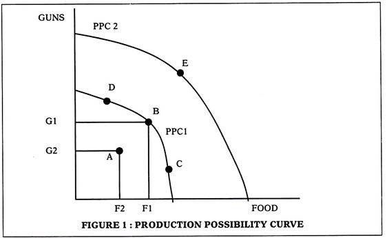
Consider two goods – food and guns as shown in figure 1. Any point on the curve PPC1 (like point B) tells us that we can produce F1 amount of food and G1 amount of guns. We can also be at any point inside the curve like A, where F2 food and G2 guns are produced. We cannot be at any point outside the curve as such points (point E) are unattain­able. This is because we do not have the resources to produce at such points. If technology improves and/or resources increase we will see the PPC shift outwards as shown. The point E is now attainable with new resources and technology as it lies on PPC 2.

The PPC Assumes the Following:

1. Technology remains unchanged when a PPC is drawn. All combina­tions that are on PPC depend on technology used and available. A new technology that is better will cause PPC to shift out to PPC 2.

2. Resources are fixed for every PPC. This means that each PPC is drawn on the basis on given level of resources. These resources refer to the total amount of resources as well as their productivity levels.

Note the Following Points that Hold for any PPC:

1. If all resources are used, we are on PPC (like point B , C, D)

2. If some resources are unused we are inside the PPC(like A)

3. Points like E are unattainable if we refer to PPC1.

4. Any change in resources causes PPC to shift. For example assume an earthquake hits a region. It will cause a decline in number of workers available, which are a resource. This will cause an inward shift of the PPC.

5. Any increase in productivity of resources and/or better technology will shift the PPC outwards, as shown by PPC 2.

Productive efficiency is achieved when we are at any point on the PPC. A point like A, which is inside the PPC, is productively inefficient. A point like B or C or D is productively efficient as they lie on the PPC. These points are Pareto efficient as we cannot increase production of one good, without reducing production of the other good. Consider points B and C, both of which are efficient.

If we want to move from B to C then we must reduce guns and increase food. This move from B to C is not a Pareto improvement as it entails reduction in production of guns, to increase food production. Thus, there is no Pareto improve­ment possible if we start of any of these points that lie on the PPC.

This implies that all points on PPC are Pareto efficient and no point is better than any other point. But if we move from a point inside the curve to a point on the curve then it is a Pareto improvement. Consider a move from A to B, which is a Pareto improvement as production of both food and guns rises.

It is important to note the shape of the curve as it cannot take any shape at random. Based on the assumptions we made for drawing PPC, it is bow shaped. This means that to produce more of food we must reduce gun production. This is because resources are fixed. To produce more food, we have to pull out resources (like labour) from gun factories and put them on the fields.

Consider figure 2. Assume that we want to increase food production. We want to move from B to C. Since all the resources are already used up (as we are on the curve already) we have to free up some land. This land will have to come from the land used for gun production.

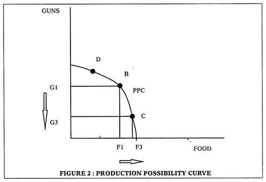
So a factory for guns may have to be shut down for freeing up land. This implies fall in gun production as the factory shuts down. To increase production of 1 good (shown by the arrow on X axis) we must reduce production of the other good (shown by the arrow on Y axis). This causes the bow shape of the PPC.

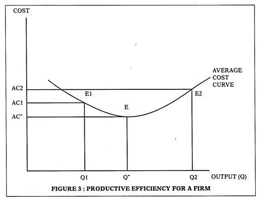
While the PPC looks at the economy from a ‘macro’ perspective, we can define productive efficiency at micro level for a firm also. A firm achieves productive efficiency when it produces at the lowest cost level. If the average cost is minimized for a firm at point E in figure 3, then it is a point of productive efficiency. Note that each firm acts in its own self-interest to minimize costs and achieve productive efficiency.

For those of us who are familiar with Microeconomics, we know that typical cost curves for any firm are U shaped. With output on the X axis and costs on the vertical axis, we can show that a productive effi­cient point for a firm to be E. This is the point where average costs are minimum. The efficient output level is Q* and average cost is AC*. At any other point (like E1) average cost is higher (AC1 > AC*). If a firm produces less than Q* it is productively inefficient. This concept applies to an output level that exceeds Q* also. At E2 average cost is AC2 while output is Q2. Note that AC2 > AC*. This makes E2 also inefficient. (See Figure 3)

2. Allocative Efficiency:

Till now we looked at efficient levels of production/output of differ­ent goods produced in an economy. Allocative efficiency takes a step backwards, to look at behind the scenes of production and considers the distribution and allocation of resources used for achieving these output levels. Let us consider figure 4, which is a simple PPC that we borrow from figure 1. Note that E1 and B are both on the PPC which qualifies them as productively efficient.

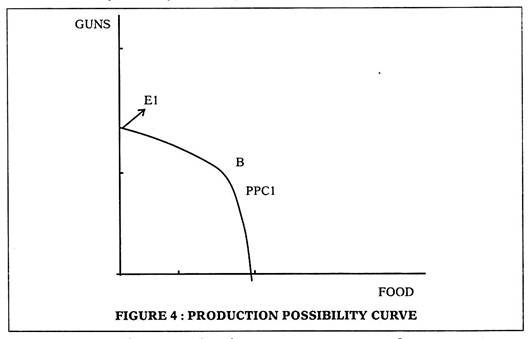
However, despite such efficien­cy El involves zero food production. All resources are devoted to gun production, and we have no food. The economy cannot live without food, which makes El a little difficult to imagine as efficient. A point like B where both guns and food are produced is more realistic and also efficient in a productive sense.

Devoting all resources to guns does not ‘seem’ correct or in the best welfare of society, (though gun makers will be really happy!). This is where allocative efficiency comes in. It looks beyond production levels and associated costs alone, and looks towards benefits of any activity, in marginal terms.

To understand this, consider that we want to get to the nearest Metro station. We have 2 options – to walk for 10 minutes or hire a rickshaw that takes 5 minutes. In making a choice, we are comparing both modes of transport in terms of the cost involved and the advantages (or benefits).

Using a rickshaw saves time (which must be considered as a benefit), but involves a price that we pay to the driver of the rickshaw (which is a cost of this option). We know that the cost is (assume) Rs.20, but we must put a monetary value to the time we save. This value depends on individual preferences.

A person who has an interview in the next hour will assign a value of Rs.100 to the time saved, while another person who has no appointments may assign only Rs.10 to the time saved. In this case, the net benefits= 100 – 20 = 80 for the person who has an interview or 10 – 20 = -10 for the person with no appointment.

On the other hand, walking costs us time but give health benefits. The cost of walking is the time we spend on it. Suppose it takes 10 minutes for any person to walk to Metro. The cost of 10 minutes again depends on individual preferences. For the person who has an interview this time is more valuable than for the person with no appointments. In the same way the value of benefits can vary across people.

The man with an interview would not like to miss it so he may value health benefits at only Rs.5. This gives net benefits of 5 – 100 = -95 to him. If he now compares the 2 options he has net benefits of +80 from using a rickshaw and net benefits of -95 from walking. Common sense dictates that he will choose to use the rickshaw.

The above example was discussed to illustrate that each decision we take involves comparing costs and benefits to arrive at net benefits from each option available to us. We choose the option with higher net benefits. The difference in some people opting for rickshaw or walking is the value they assign to benefits and costs. The differences in these valuations lead to different choices when two people are faced with same options

Every person attributes a different value to the cost and benefits to options available. A calculation of net benefits (= benefits – costs) is done. The option with highest net benefits is taken by a rational person.

The same logic applies in Microeconomics – any economic activity must be done if the marginal benefit from that activity exceeds or equals its marginal cost, or net marginal benefits are positive. If two activities are given and one has to be chosen then the activity with higher net mar­ginal benefits must be done. The use of the word marginal is done as we compare costs and benefits of the last unit of output. The decision is always about the next unit – to produce or not produce.

Rule-to Produces any Good Marginal Benefit ≥ Marginal Cost for the Last/Marginal Unit of a Good:

This rule needs a calculation of costs and benefits of any activity. While costs of any productive activity are easy to calculate in terms of the wages, inputs and other resources that are used to produce it, the measurement of benefits is not so easy. Benefits can be subjective. Consider the same employees who are faced with an option of buying a pair of shoes.

Vineet may like the pair of shoes more than Radhika. This is shown in the fact that he is willing to pay more than Radhika for the shoes. Price is therefore, used as a reflection/representative of the marginal benefit we derive, as it tells us what we are willing to pay for the marginal unit. Net benefits will be price – costs of producing the shoes. Allocative efficiency requires that Price= Marginal Cost for each good produced in the economy. Goods are produced till net benefits equal zero for the last unit produced.

In real life, a firm will have to consider both types of efficiencies. It must combine its inputs in a manner that minimizes costs to achieve productive efficiency. It must set a price of the good it sells in a way that maximizes revenues/profits for itself. These efficiencies are not always achieved as a firm does not have an objective that is based on efficiency.

In most markets a firm may choose to ignore allocative efficiency, in order to maximise its profits. Consider a monopolist firm that seeks profit maximization. Economic theory dictates that the optimal price will not equal the marginal cost of producing the unit, causing alloc­ative inefficiency.

This is because profit maximization dictates that price exceeding the marginal cost for a good. Thus, a monopoly firm may achieve productive efficiency, but will always be allocatively inefficient in equilibrium. The other end of the spectrum in market forms constitutes perfect competition.

In a perfectly competitive structure, both efficiencies are achieved, which is why it is like an ‘ideal’ market structure. This also leads to maximum welfare for all economic agents taken collectively.

The next question is – perfect competition is rare in real life, and we have some imperfectness in markets which increases allocative inefficiency. How can we ensure allocative efficiency is achieved by firms in real life?

An obvious answer is to let government or any agency ‘force’ a firm to sell at a price that equals marginal cost, so that then we have allocative efficiency along with productive efficiency. However, this is not in the self-interests of a profit seeking firm, as profits will not be maximum when P = MC. Also enforcement of such rules may be cost ineffective and breeds corruption. Thus, in real life the self-interest (of maximizing profits) causes firms to achieve productive efficiency, while allocative efficiency is only a feature of perfect competition.

We can illustrate allocative efficiency using the PPC framework also. Consider two goods in the economy again in figure 5. For allocative effi­ciency we need MC1= P1 and MC2= P2

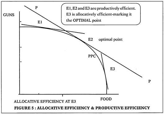
This is also expressed as MC1/MC2= P1/P2. This is shown on the PPC in terms of tangency at a point. Consider 3 points- E1, E2 and E3, all of which lie on the PPC so that all are productively efficient. The price ratio is shown by the slope of the price line PP. The slope of the PPC denotes ratio of marginal costs. The slope of the PPC at points E1 and E2 show the ratio of marginal costs-

1. At E1 we can see that slope of PPC > slope of price line. This implies that MC1/MC2 > P1/P2, making this point allocatively inefficient. Costs outweigh the benefits.

2. At E3 we can see that slope of PPC < slope of price line. This im­plies that MC1/MC2 < P1/P2, making this point also allocatively inefficient. The prices are higher than the benefits at this point.

3. At E2 we can see that slope of PPC = slope of price line. This implies that MC1/MC2 = P1/P2, making this point allocatively efficient as ratio of marginal prices equal ratio of marginal costs. Point E2 is therefore both productively and allocatively efficient.

We can have many other types of efficiencies in the system. Some of them include social efficiency, X efficiency and dynamic efficiency, but these are beyond the scope of this course.