LM-Curve: Derivation, Factors, Situations, Interpretation!
Money Market Equilibrium: The LM Curve:
The Derivation of the LM Curve:
The Keynesian demand function for money is expressed as
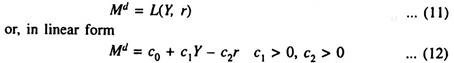
Here c0 is the intercept of the money demand function, c1 is the increase in money demand per unit increase in Y, and c2 is fall in money demand per unit increase in r.
ADVERTISEMENTS:
It may be recalled that transactions demand for money in the Keynesian model is assumed to depend positively on income and speculative demand and inversely on the rate of interest.
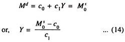
The money market is in equilibrium when the demand for money indicated by symbol L (equation 10) is equal to the fixed (exogenously determined) supply of money:
M0S = Md = c0 + c1Y – C2r …(13)
ADVERTISEMENTS:
In order to derive the LM curve which shows money market equilibrium, we have to find combinations of r and Y that equate money demand with a fixed money supply. The LM curve is a locus of points showing all combinations of r and Y which equilibrate the money market.
Fig. 9.13 shows how the LM curve is derived. Part (a) shows that increases in income (from Y0 to Y1 to Y2) shift the demand curve for money from Md(Y0) to Md(Y1), then to Md (Y2). In order to restore equilibrium in the money market, the rate of interest has to rise from r0 to r1 and r2 as income increases from Y0 to Y1 and to Y2.
In part (b) we derive the LM curve by connecting points like E, E’ and E” showing combinations of income (K) and the interest rate r that equilibrate the money market. Points E, E’ and E” showing equilibrium combinations such as (r0, Y0), (r1, Y1,) and (r2, Y2) in part (b) correspond to the same points in part (a). Part (a) shows that as income increases, higher interest rates are required for money market equilibrium.
This is why the LM curve is upward sloping from left to right. In part (a), when the money market is in equilibrium at point E, money demand equals money supply at the equilibrium interest rate, r0. This corresponds to point E on the LM curve in part (b), showing money market equilibrium, with Y = Y0 and r = r0.

In part (a), as income increases from Y0 to Y1, and to Y2 the demand for money increases and the demand curve for money shifts upward parallely. As a result the rate of interest rises from r0 to r, and from r1 to r2 as shown by points E’ and E”. These three points of money market equilibrium in part (a) correspond with points E, E’ and E” which lie on the LM curve showing three combinations of Y and r, viz., Y0 and r0, Y1 and r1 and Y2 and r2.
Thus we see that the LM curve is a locus of points showing alternative combinations of Y and r that bring about money market equilibrium. The LM curve is upward sloping from left to right because as the level of income rises higher interest rates are required to reachieve money market equilibrium.
Now we have to know two things about the LM curve. Firstly, we must know what determines the steepness (or flatness) of the curve because the slope of the curve determines the effectiveness of stabilisation policies. Secondly, we have to know which factors shift the LM curve. These two issues may now be taken up one by one.
i. Factors Determining the Slope of the LM Curve:
The steepness or flatness of the LM curve depends on interest elasticity of demand for money. If the demand for money is interest inelastic the LM curve will be fairly steep. If it is fairly elastic, the LM curve will be relatively flat.
The higher the value of c1, the steeper the LM curve. The reason is that the higher the value of c1, the larger the increase in money demand per unit increase in income, and hence, the larger is the upward adjustment in the interest rate required to restore money market equilibrium. The higher is c1, the steeper will be the LM curve.
If money demand is highly interest elastic (c2 is large), a relatively small increase in the interest rate will offset the increase in transactions demand for money caused by a rise in income from Y0 to Y1 and to Y2 if c1 (which shows the increase in M per unit increase in income) remains constant.
In Fig. 9.14(a) the interest elasticity of demand for money is low (in absolute value). This is why the demand curve for money is relatively steep. In this case, the LM curve is also (a) Low Interest Elasticity of Money Demand relatively steep. In Fig. 9.14(b) we show an almost opposite type of situation.
Since the demand for money is higher interest elastic (i.e., responsive to interest rate changes), the demand curve for money is relatively flat. In such a situation the LM curve is also relatively flat.

Two Extreme Situations:
A. The Classical Case:
If the interest elasticity of demand for money is zero (c2 = 0) as in the classical model which does not consider speculative demand for money, we get the following equation of the LM curve
Thus, only this level of income can be the equilibrium level for the money market and the LM curve is vertical, as shown in Fig. 9.15.

B. The Liquidity Trap Case:
Another extreme situation is one in which the speculative demand for money is infinitely elastic at a very low interest rate — the Keynesian liquidity trap case. At very low levels of income such as Y0 and K, equilibrium in the money market in part(a) of Fig. 9.16 occurs at points such as E and E’ along the flat portion of the demand curve for money where the elasticity of money demand is extremely high.
ADVERTISEMENTS:
Consequently the LM curve in part(b) of Fig. 9.16 is almost horizontal over this range of income. At higher income levels such as Y2 and Y3, money market is in equilibrium at steeper points F and F’ along the demand curves for money such as Md(Y2) and Md(Y3). So the corresponding LM curve is steep, because interest elasticity of demand for money is low.
Since the economy is not in a liquidity trap situation, an increase in income would require a large increase in the interest rate to restore money market equilibrium.

i. Factors Shifting the LM Curve:
Two factors shift the LM curve — a change in the supply of money and a change in the demand for money (liquidity preference). We first show the effect of money supply change which occurs due to change in the central bank’s policy. Solving the equation of the LM curve for the interest rate enables us to identify the intercept and slope of the LM curve. Since M0S = c0 + c1Y – c2r we get
ADVERTISEMENTS:
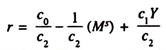
Since the intercept of the LM curve contains the money supply (MS0 ) any time money supply increases (decreases) the intercept will shift up (down) and the LM curve will shift up (down). Fig. 9.17 shows the effect of an exogenous increase in money supply on the LM curve.
In part (a), the money market is in equilibrium at point E. If money supply increases from Ms0 to M1s the rate of interest falls from r0 to r1 (at a given level of income Y0) as the money market reaches new equilibrium at point F.

As a result the LM curve shifts to the right, indicating lower interest rates at all levels of income.
In short, an increase in the money supply shifts the LM curve downward and to the right. The converse is also true. A fall in money supply will shift the LM curve upward and to the left.
ii. Shifts in the Money Demand Curve:
ADVERTISEMENTS:
If the demand for money increases (falls) the LM curve shifts to the left (right). Suppose due to some reason, such as people’s loss of confidence in bonds the demand for money increases at the same level of income and the same rate of interest.
As a result, the demand curve for money shifts upward and to the right from M0d (Y0) to M1d (Y0) in Fig. 9.18. As a result, the equilibrium rate of interest rises for the same level of income (Y0) in part (a). Consequently the LM curve shifts upward and to the left from LM0 to LM1 in part (b).

The Quantity Theory Interpretation of the LM Curve:
We know that the theory behind the upward sloping LM curve is Keynes’ liquidity preference theory. But it is also possible to derive the LM curve by adopting the Quantity Theory approach. The quantity equation of exchange MV = PY gives us the equilibrium condition of the money market.
If V is assumed to remain constant, the equation is converted into the quantity theory of money. The assumption implies that, for any given price level P, the supply of money M itself is determined by the level of income Y:
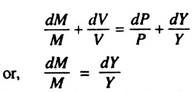
Since the level of income does not depend on r, the LM curve derived from the quantity theory is vertical. See Fig. 9.19(a).
ADVERTISEMENTS:
However if we relax the assumption of constant. V, we get the more familiar upward sloping LM curve from the quantity equation. The assumption that V = V̅ implies that the demand for real money balances depends only on Y. However, in Keynes’ theory, the demand for real money balances also depends on r : a high r raises the cost of holding money and reduces the demand for money.
If r rises, people reduce their money holding. So they use each rupee more frequently to buy a certain fixed amount of goods and services (or to support a given volume of transactions). Thus V increases when r rises. So we now express velocity as a function of r:
![]()
Here V is positively related to r. Since an increase in r raises V, it also raises Y, if M and P remain constant. In this case the LM curve will upward sloping due to a positive relationship between r and Y which originates from the money market. See Fig. 9.19(b).
 Equation (a’) also shows that any change in M will shift the LM curve. For any given interest rate and price level, the money supply and the level of income move up or down at the same time. Thus increases in M shift the LM curve to the right and decreases in M shift the LM curve to the left.
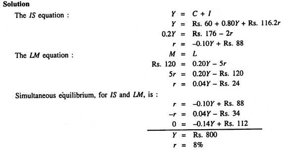
Example:
ADVERTISEMENTS:
1. In a two-sector model, suppose C = Rs. 60 + 0.80Y, I = Rs. 116 – 2r, L = 0.20Y – 5r and M = Rs. 120. Find out the equilibrium values of Y and r.