
Here is a compilation of essays on ‘Demand’ for class 9, 10, 11, and 12. Find paragraphs, long and short essays on ‘Demand’ especially written for school and college students in Hindi language.
Essay on Demand
Essay Contents:
- Essay on Introduction to the Theory of Demand
- Essay on Market Demand and Aggregation Problem
- Essay on Properties of the Demand Function
- Essay on Market Demand and Elasticity
- Essay on Determinants of Price Elasticity of Demand
- Essay on Income Elasticity of Demand
- Essay on Cross Elasticity of Demand
- Essay on Theoretical Foundations of Demand
Essay # 1. Introduction to the Theory of Demand:
ADVERTISEMENTS:
The theory of demand was mostly implicit in the writings of classical economists before the 19th century. Current theory rests on the foundations laid by A. Marshall (1890), F.E. Edge worth (1881) and V. Pareto (1896). Marshall viewed demand in a cardinal context, in which utility could be quantified.
Most contemporary economists hold the approach taken by Edge worth and Pareto, in which demand has only ordinal characteristics, and in which indifference or preference becomes central to the analysis It is against this backdrop that we study the theory of consumer demand. The theory of consumer demand can be studied at two different levels, viz., at the individual level and at the aggregative (market) level.
The starting point of the theory is the demand function which is a multivariate relation We derive the downward sloping demand curve for a normal good of individual consumer by making the ceteris paribus assumption, i.e., holding all the variables except the price of the commodity constant.
If there is a change in the price of the commodity under consideration there is movement along the same demand curve. The law of demand states that the consumer responds to lower prices by buying more.
ADVERTISEMENTS:
There are various exceptions to the law of demand. The best known exception is the Giffen good—a consumer buys more, not less, of a commodity at higher prices Another is the Veblen effect-some commodities are wanted solely for their higher prices.
The higher these prices are, the more the use of such commodities fulfills the requirements of conspicuous consumption, and thus the stronger the demand for them. However, if there is a change in any other variable except the price of the commodity the whole demand curve shifts to a new position (implying change in demand, i.e., change in the conditions of demand).
Essay # 2. Market Demand and Aggregation Problem:
However, for analytical purposes, what is relevant is market demand and not individual demand. The reason is that the price of a commodity is determined not by individual demand but by market demand. The market demand for a commodity is derived by adding up the demand curves of individual consumers.
ADVERTISEMENTS:
However, three aggregation problems arise while arriving at the market demand curve by horizontally adding up individual demand curves, viz.,
(i) The snob effect,
(ii) The bandwagon effect (also known as network externality) and
(iii) The Veblen effect.
Essay # 3. Properties of the Demand Function:
The demand function of an individual consumer has two properties. First, the demand function is single-valued, i.e., there is a one-to-one relation between a particular price and a particular quantity Second, the demand function is homogeneous of degree of zero in prices and income.
This property follows from the fact that if all absolute prices and money income of the consumer change in the same direction and in the same proportion, the consumer’s real income or purchasing power will remain unchanged. So there will be no change in the consumer s equilibrium purchase of any commodity.
This property follows from the fact that the consumer does not suffer from money illusion, i.e., he does not, through mistake, take the increase in money income as an increase in real income (purchasing power). These properties of the demand function were first brought into focus by P. A. Samuelson under the heading: meaningful theorems.
Essay # 4. Market Demand and Elasticity:
ADVERTISEMENTS:
The law of demand indicates the direction of change in quantity demanded of a commodity to a change in its own price, ceteris paribus. However, with a view to finding out the exact response of the consumer to a change in price or any other variable affecting demand Marshal introduced the concept of elasticity of demand. Elasticity of demand is a measure of market sensitivity of demand.
It measures the degree of responsiveness of consumers to a change in price of a commodity, the income of buyers or change in the price of any other commodity which may be a substitute or a complement.
Thus, elasticity is of three main types:
i. Price
ADVERTISEMENTS:
ii. Income and
iii. Cross.
Sometimes we refer to another concept of elasticity, viz., promotional elasticity or, more precisely, advertisement elasticity of sales.
Slope vs. Elasticity:
ADVERTISEMENTS:
It may apparently seem that the slope of the demand curve is the same as its elasticity. But this is a false belief. The truth is that slope measures absolute change and elasticity measures percentage change. The coefficient of price elasticity of demand (ep) is written as
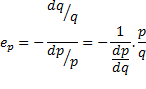
This means that the reciprocal of the slope of the demand curve (dp/dq) has to be multiplied by the original price-quantity ratio to find out the numerical value of ep. Only in two extreme situations it is possible to measure price elasticity demand from the slope of the demand function alone, viz., the case of completely elastic demand, and the case of completely inelastic demand. If the demand curve is horizontal, its slope is zero but elasticity is infinite. But if the demand curve is vertical its slope is infinite but its elasticity is zero.
Price elasticity of demand falls along a straight line demand curve, even if its slope remains the same at all points. By contrast, if the demand curve is a rectangular hyperbola its slope changes from point to point but its elasticity is the same at all points.
Essay # 5. Determinants of Price Elasticity of Demand:
There are various determinants of price elasticity of demand. Perhaps the most important determinant is the number and closeness of substitutes available. This, in its turn, depends on the definition of the commodity.
ADVERTISEMENTS:
The demand for chocolates, for example, is fairly inelastic, because for those who are very fond of chocolate there is no substitute. But the demand for a particular variety of chocolate, such as Amul chocolate, is elastic because substitutes are readily available.
There is an important theorem on price elasticity of demand.
Theorem:
If two goods are neither substitutes nor complements, the sum of partial price elasticity’s of demand is zero with a negative sign.
Essay # 6. Income Elasticity of Demand:
Income elasticity of demand measures the degree of responsiveness of the demand for a commodity to a change in the income of the buyers, holding prices of different purchasable goods and other variables affecting demand (such as the taste and preference of buyers) constant.
ADVERTISEMENTS:
On the basis of the value of the coefficient of income elasticity of demand we can classify goods into two main categories—normal (having positive income elasticity of demand), and inferior (having negative income elasticity of demand). It may be noted that inferiority has nothing to do with the physical property of a commodity.
Inferiority is related to the income position of the buyer. If the consumer’s demand for a good falls when his income increases, it is called an inferior good. In case of a superior (luxury) good the coefficient of income elasticity is greater than one, in case of a normal good it is less than one, and it is negative in case of an inferior good.
There are two important theorems on income elasticity of demand:
Theorem 1:
The sum of the expenditure share weighted income elasticities of demand is equal to 1. This means that if one good is a luxury the other must be an inferior one. However, if the consumer spends all his income on two goods both cannot be inferior luxury at the same time, but both can be normal.
Theorem 2:
ADVERTISEMENTS:
If income elasticity of demand of all the goods is equal, then also the sum of the income elasticities will be equal to 1.
Essay # 7. Cross Elasticity of Demand:
The quantity demanded of a commodity depends not only on its own price but also on the prices of other goods which compete for a limited amount of the consumer’s budget. Cross elasticity of demand measures the degree of responsiveness of the quantity demanded of a commodity to a certain percentage change in the price of another commodity.
On the basis of the value of the coefficient of cross elasticity of demand we can classify commodities into three categories, viz., substitutes (with positive cross elasticity), complements (with negative cross elasticity) and unrelated goods (with zero cross elasticity).
Relation among the Three Elasticities:
The sum of the partial price, cross and income elasticities of demand is zero. This can be proved by using the Euler’s theorem.
ADVERTISEMENTS:
Elasticity of Market Demand Curve:
The market demand curve for a commodity is more elastic than that of an individual consumer. The reason is that when price of a commodity falls, three effects are generated simultaneously. First, existing consumers buy more of the commodity. Second, price fall brings new consumers into the market since potential buyers become actual buyers. This is known as the market size effect. Third, when the price of a commodity falls, people develop
Essay # 8. Theoretical Foundations of Demand:
Economists have found it more interesting to study individual demand than market demand. In this context they have built the theoretical foundations of demand. We study theory of consumer demand with a twofold objective. Our first objective is to find out the equilibrium condition of a rational consumer whose objective is utility (welfare) maximisation subject to the budget (income) constraint. Our second objective is to derive the demand curve of the consumer and account for its negative (downward) slope.
Two main approaches to the theory of consumer demand are the cardinal (utility) approach and the ordinal (indifference curve or preference) approach. The second variant of the ordinal approach is known as the revealed preference approach. These approaches may now be reviewed.
i. The Cardinal (Utility) Approach:
Marshall develops the cardinal approach by bringing into focus the distinction between marginal utility and total utility. The classical economists like Adam Smith, David Ricardo and others were surprised by the fact that the price of water (which was so essential for an individual’s existence) was less than the price of diamond (which was a non-essential or a luxury good the possession of which gave only psychic satisfaction to the consumer). So a paradox was encountered, known as the paradox of value or the water-diamond paradox.
The paradox was resolved by Marshall by using the concept of marginal utility. According to Marshall, the price of a commodity is determined from the demand side, not by total utility, but by marginal utility. Since marginal utility of diamond is higher than that of water, the price of diamond is higher than the price of water.
Marshall developed the cardinal (utility) approach by assuming that utility can be measured or quantified. So his approach is based on the concept of measurable utility. He assumes that the utility of commodity can be measured in cardinal numbers, called utils.
He also assumes that the marginal utility of money remains constant at all levels of income. On the basis of this assumption Marshall developed the equilibrium condition of the consumer in terms of a famous law, known as the law of equimarginal utility which is expressed as
![]()
where λ is the constant marginal utility of money. If this assumption (i.e., constancy of λ) is violated the law will not hold. The law simply states that the ratio of marginal utility to price has to be same for all goods and all such ratios must be equal to the constant marginal utility of money.
The Downward Slope of the Demand Curve:
According to Marshall the demand curve for a normal good is downward sloping due to the operation of a fundamental psychological law, viz., the law of diminishing marginal utility. The marginal utility of a commodity indicates the maximum amount the consumer is willing to pay to buy one extra unit of a commodity.
As the consumption of a commodity increases the consumer s psychological inclination or capacity to appreciate every extra unit of it gradually falls.
As marginal utility falls, the consumer is ready to pay less and less price to acquire every extra unit of it. This means that price change and quantity change of a commodity are in the opposite direction. And the demand curve of a normal good slopes downward from left to right.
The Marshallian demand curve is called ordinary demand curve. The reason will be explained later in this essay in the context of the ordinal approach to the theory of demand.
Two Implications of the Marshallian Approach:
1. By using the cardinal approach Marshall developed the concept of consumer surplus It is’ utility surplus and not monetary surplus. So it cannot be measured in a meaningful way However, the only prediction we can make is that price fall leads to an increase in consumer surplus and a price increase leads to a fall in consumer surplus.
In spite of this, the concept has a number of practical uses. For example, the concept is used to show the net welfare loss from an indirect tax called deadweight loss. Similarly, there is welfare loss in monopoly because a monopolist takes away the entire consumer surplus and converts this into his own profit.
2. Marshall assumes that utility function of an individual is separable and is written as
u (x1, x2, x2) =f1(x1) +f2(x2) +f3(x3)
where f1 (x1) i= 1, 2, 3. If the utility of each good is independent of the quantity of other goods, then all goods must have positive income elasticities. Thus, the Marshallian approach rules out the existence of inferior goods.
Criticisms of the Marshallian Approach:
Two main criticisms of the cardinal approach are:
(i) Utility is a subjective concept and cannot be objectively measured.
(ii) The marginal utility of money does not remain constant at all levels of income. So the law of diminishing marginal utility does not hold.
In order to remove these two defects of the cardinal approach, initially Pareto and Edge worth and, subsequently, J.R. Hicks and R.G.D. Allen, developed the ordinal or indifference curve approach to the theory of consumer demand. Since this approach is based on the taste and preference of the buyer, it is also called the preference approach.
ii. The Indifference Curve (Preference) Approach:
In order to develop a meaningful theory of consumer demand we need three pieces of information, viz:
(i) The taste and preference of the consumer,
(ii) His money income, and
(iii) The prices of the purchasable goods.
Information about (i) is given by indifference curves, which is a nice way of summarizing a consumer’s taste. Information about (ii) and (iii) is given by the budget line.
The budget line is so important for the consumer because in his search for maximum utility, the consumer is faced with a budget (or an income) constraint. And a rational consumer is supposed to maximise utility (welfare), subject to the budget constraint.
While an indifference curve shows the consumer’s desire (willingness) to buy certain goods, the budget line shows his capacity (power) to buy such goods. And the consumer reaches equilibrium when his desire to buy coincides with his capacity, i.e., when he ends up buying exactly what he intends to buy. The indifference curve approach is based on a number of axioms such as the consistency, rationality, non-satiety and dominance.
The indifference curve approach proceeds in three steps:
Step 1: Definition and Properties of Indifference Curves:
An indifference curve is a locus of points showing alternative combinations of any two goods which yield the same level of satisfaction to the consumer, as shown in Fig. 1. An indifference curve is a boundary line separating the superior points (points above an IQ from the inferior points (points below IC). An indifference curve may also be called an iso-utility curve.

In a commodity space, like the one shown in Fig. 2 we can draw any number of indifference curves such as IC1, IC2 and IC3. All the indifference curves together constitute the indifference map of the consumer. In other words, the indifference map is the collection of all indifference curves.

Indifference curves have five important properties:
1. Density:
Indifference curves are always dense, i.e., in a particular commodity space we can draw any number of indifference curves.
2. Preferred Combination:
An indifference curve which lies above and to the right of another such curve shows a preferred combination of the two commodities. This means that any point on a higher indifference curve (such as IC2 in Fig. 2) is better than that on a lower indifference curve (IC1).
3. Negative Slope:
An indifference curve slopes downward from left to right. This is due to the law of substitution which states that the consumption of one good is always at the expense of the other. If the consumption of a commodity falls, the consumer requires more of another commodity as compensation so as to prevent his utility from falling. On a particular indifference curve such as IC1 in Fig. 3 we find that at a point like E
![]()
![]()

This is known as the marginal rate of substitution of x1 for x2 (MRSX1 X2) or the desired rate of commodity substitution. It is the rate at which the consumer wants to substitute one commodity by the other while staying on the same indifference curve and enjoying the same level of satisfaction or utility. It is the ratio of the two marginal utilities.
However, measurement of marginal utility is not necessary for measurement of MRS. In fact, the concept of utility has no relevance in the modern theory of consumer demand’ except in situations involving choice under uncertainty.
4. Intersecting ICs:
Two indifference curves cannot meet or intersect. In other words one must lie consistently above or below another. Otherwise the consistency axiom will be violated
5. Convexity:
An indifference curve is convex since an averaged bundle is assumed to be better than an extreme bundle. However, diminishing marginal utility is neither necessary nor sufficient for the convexity of indifference curves.
Step 2: The Budget Line:
The budget line shows the consumer’s capacity to buy different combinations of any two goods at prevailing market prices. It is also called the consumption possibility line. It is expressed as
M = p1x1 +p2x2
where all the terms have their usual meaning and its slope is P1 /P2 which is the price ratio or the actual rate of commodity substitution. The budget line is shown in Fig. 4 as the straight line AB. All the points inside the budget line or on the budget line are attainable points.
However, a point like U outside the budget line is an unattainable point. This means that a consumer with a fixed income (m) and facing a fixed set of commodity prices (p1 and p2) can stay on the budget line or inside the budget line but he cannot go beyond the budget line.

Step 3: Consumer Equilibrium:
A rational consumer whose objective is utility maximisation will always try to reach the highest attainable indifference curves permitted by the budget line as shown in Fig: 5. Here the consumer reaches equilibrium and maximises welfare at point E were the MRS (or the desired rate of commodity substitution) is the same as the price ratio (or the actual rate of commodity substitution).

The Consumer’s Reaction to Income and Price Changes:
If the consumer’s money income alone increases (decreases) the budget line shifts to the right (left) This enables the consumer to reach higher and higher (lower and lower) indifference curves and enjoy more utility (satisfaction). The locus of successive equilibrium points such as E, F and G in Fig. 6 is known as the income consumption curve (ICC). If both goods are normal the ICC will be upward sloping.
If any of the two goods is an inferior one, the ICC may be backward bending or forward falling. This means that in a two-commodity world, both cannot be inferior at the same time. From the ICC or the income expansion path we can derive the Engel curve or income demand curve. The Engel curve for an inferior good is backward bending.

If there is a fall in the market price of one of the purchasable goods, the budget line becomes flatter. This enables the consumer to reach a higher indifference curve and enjoy more utility or satisfaction. The locus of successive equilibrium points is called the price consumption curve (FCC). It shows the consumer’s reaction to a change in the market price of x1, as shown in Fig. 7.

Two Uses of PCC:
1. From the PCC we can derive the consumer’s demand curve for a good such as x1. However if indifference curves are not convex throughout, the demand curve will be discontinuous.
2. From the PCC we can predict price elasticity of demand on the basis of the total outlay method:
(i) If PCC is downward sloping, ep>1;
(ii) If PCC is horizontal, = 1; and
(iii) If PCC is upward sloping, ep < 1.
Price Effect as the Sum Total of SE and IE:
It was initially E. Slutsky and then J. R. Hicks who decomposed the (total) effect of a fall in the price of a commodity such as x1 into two parts—the substitution effect and the income effect. This exercise was not done by Marshall. This is why the Marshallian demand curve is known as the ordinary (uncompensated) demand curve. Slutsky and Hicks developed two different approaches to measure the substitution effect.
While Hicks’ substitution effect is measured by holding total utility constant, Slutsky substitution effect is measured by holding real income constant. While measuring substitution effect, income effect is first eliminated. This is why the Hicks and Slutsky demand curve are called compensated demand curves.
So there are three types of demand curves:
1. Marshallian demand curve (called money income constant demand curve);
2. Hicks compensated demand curve (called total utility curve demand curve);
3. Slutsky compensated demand curve (called real income constant demand curve).
The ordinary demand curve is more elastic than compensated demand curve due to elimination of income effect. And, of the two compensated demand curves, the Slutsky compensated demand curve is more elastic than the Hicks compensated demand curve.
Price effect is the sumtotal of substitution effect and income effect. If two goods are perfect substitutes, such as blue ink and black ink, for a colour blind person the indifference curves are straight lines. In this case price effect is equal to substitution effect and income effect is zero. By contrast, if two goods are perfect compliments then price effect is equal to income effect and the substitution effect is zero.
Substitution effect is always negative for convex indifferent curves’. Income effect is also negative in case of a normal good (if we consider change in real income). So the price effect is negative and is quite strong since the two effects go in the same direction. However, income effect is positive in case of an inferior good but is less stronger than the negative substitution effect.
So the price effect is still negative, and the demand curve of an inferior good is downward sloping but steeper than that in the case of a normal good. In case of a Giffen good (which is a special variety of inferior good) the positive income effect is stronger than the negative substitution effect. So the price effect is positive and demand curve of a Giffen good is upward sloping. This is an important exception to the empirical law of demand.
Two related points may also be noted in this context:
1. The compensated demand curve is downward sloping even in case of a Giffen good.
2. An inferior good is an income phenomenon but a Giffen good is a price phenomenon.
Applications of Indifference Curves:
Indifference curve and budget lines can be used to throw light on a number of real life issues:
1. First, we can show the welfare effects of taxes and subsidies. To be more specific, it is possible to show the alleged superiority of income tax over sales (excise) tax.
2. We can also show that a gift-in-cash is better than a gift-in-kind (e.g., food stamp).
3. If the consumer spends all his income on one good, we get a corner solution (called monomania). This happens if indifference curves are concave or if the highest attainable indifference curve is steeper than the budget line except at the corner point.
4. In addition, indifference curves and budget lines can be used to show inter-temporal choice—consumption smoothing overtime through borrowing and lending.
5. Income and substitution effect can also be used to show labour-leisure choice of an individual and to account for the backward bending labour supply curve of an individual worker It can also be shown that while a straight wage increase (i.e., wage increase for all the hour worked) generates both income effect and substitution effect, a rise in overtime wage generates only substitution effect. Therefore, the labour supply curve is upward sloping in case of a rise in overtime wage.
6. It is also possible to prove the homogeneity property of the demand function in a two- commodity world by using the Lagrange multiplier method or the graphical method. The homogeneity property holds in case of balanced price and income changes.
7. Utility curves can be used to show choices under uncertainty. The curvature of the utility functions shows an individual’s attitude towards risk.
8. However, we can also use indifference curves in case of a risk-return choice. Such indifference curves are upward sloping from left to right.
9. If both the commodities are economic bads, the indifference curves would be concave rather than convex. Examples of two economic bads are inflation and unemployment.
Product Characteristics Approach:
K. Lancaster has applied the indifference curves approach to develop a new theory of consumer demand, viz., the product characteristics theory. Lancaster’s product characteristics/attributes model is essentially a theory of consumer behaviour that shows how consumers choose between a number of brands of a product, each of which offers a particular product characteristic in fixed proportions. For example, a consumer buying mixed fruit juice may be looking for two principal characteristics—flavour and vitamin content.
Three brands of such juice are available—Brand A, Brand B and Brand C—each of which is differentiated insofar as it places a different emphasis on the two product characteristics. The three brands are represented by the rays in Fig. 8, each of which shows the fixed proportion of product characteristics in each brand. Brand A, for example, has high vitamin content but little flavour, while Brand C, by contrast, has a lot of flavour but a low vitamin content.

Points a, b and c on these rays show how much of each brand of juice can be bought for a given unit of expenditure at the prevailing prices of the three brands. To find the consumer’s utility-maximising brand purchases, it is necessary to introduce a set of indifference curves such as IC1, IC2 and IC3, showing the consumer’s preferences between the two product characteristics. The consumer’s final choice will be Brand B, as it settles at point b on the highest attainable indifference curve IC3 consistent with the limited expenditure.
iii. Revealed Preference Approach:
In 1938 P. A. Samuelson developed the revealed preference approach. The novelty of the approach is that it is possible to account for the downward slope of the demand curve for a commodity without using indifference curve, i.e., from the budget lines alone.
This approach is based on the behaviour of the consumer in the market place or on his actual choice. However H. Houthakkar and W.J. Baumol have shown that it is still possible to derive indifference curves by using the revealed preference approach.
The revealed preference approach provides an explanation for an individual consumer’s downward sloping demand curve, requiring him to reveal his preferences in any given set of circumstances. Like the indifference curve approach the revealed preference approach is also based on a number of axioms. The most important one is the weak axiom of revealed preference (WARP). The other one is the strong axiom of revealed preference (SARP)
In Fig. 9 we illustrate the revealed preference approach. The consumer initially is in equilibrium at point E. If the price of x1 falls the budget line becomes flatter. Now if we eliminate the real income effect by shifting the budget line to the left and parallel to itself so that it passes through point E, the new budget line is A’C’ whose slope is the same is that of AC. And the consumer moves from E to F (the substitution effect). Now if we restore the income effect by shifting the budget line back to its original position AC,the consumer moves from F to G (the income effect).

Since the consumer buys more x1 and less x2 by moving from E to F, the substitution effect is negative and the demand curve for X1 is downward sloping. The revealed preference approach is superior to the indifference curve approach since the former does not suffer from dimensional limitation. It is possible to use the revealed preference approach in case of a consumer who buys more than two goods. It is also possible to prove the homogeneity property of the demand function by using the revealed preference approach.
Moreover, quantity indices can be used to test the WARP and assess the welfare effect of price changes. One major limitation of the revealed preference approach is that by using this approach it is not possible to classify commodities into three categories-normal goods, inferior goods, and Giffen goods.