
After reading this article you will learn about:- 1. Meaning of Cost Benefit Analysis 2. Steps in Cost Benefit Analysis 3. Costs and Benefits in Controlling Pollution 4. Cost Benefit Analysis—The Frame Work 5. Merits and Demerits.
Contents:
- Meaning of Cost Benefit Analysis
- Steps in Cost Benefit Analysis
- Costs and Benefits in Controlling Pollution
- Cost Benefit Analysis—The Frame Work
- Merits and Demerits of Cost Benefit Analysis
1. Meaning of Cost Benefit Analysis:
The foundation of the method of cost benefit analysis arose from the Hicks – Kaldor criterion of efficiency maximization in 1939. The criterion of Hicks-Kaldor states that a project or activity merits consideration or remains desirable when the total benefits exceed total cost.
ADVERTISEMENTS:
The cost benefit analysis states that if the benefit arrived from the pollution elimination programme is greater than the benefit received from it, it is called ‘positive benefit’. On the other hand if the cost incurred in that programme is greater that the benefit received from it, it is termed as ‘negative benefit’.
The cost benefit analysis is the tool generally undertaken by the government for the welfare of the entire society. So it is also referred as social benefits. Cost benefit analysis may be summed as ‘the cost benefit analysis which involves measuring, adding up and comparing all the benefits and all the cost of a particular public project or a programme.’
2. Steps in Cost Benefit Analysis:
Different Steps in Cost Benefit Analysis:
Before entering into the cost benefit analysis we shall see the various steps taken in this analysis.
ADVERTISEMENTS:
(i) Specify clearly the project or programme.
(ii) Describe quantitatively the inputs and outputs of the programme.
(iii) Estimate the social cost and benefits of these inputs and outputs.
(iv) Compare these benefits and costs.
ADVERTISEMENTS:
(i) Specify Clearly the Project or Programme:
The first step is to decide on the perspective from which the study is to be done. Cost benefits are actually concerned with the public. When we have decided on the perspective, the main elements of the projects such as, the study of the location, timing, groups involved, the connection with other programmes etc.
Should be considered. Again the pollution control phenomenon is a worldwide concept. So the regional planning agencies should give particular stress on the area of the study.
When the project is fixed the following two programmes are involved:
(a) Physical project:
This implies the projects like the public waste treatment plants, beach restoration projects, hazardous waste removal, habitat improvement projects, land purchase for preservation etc. These projects are physical in nature, which is done when an area is polluted.
(b) Regulatory projects:
This implies the enforcement of environmental laws and regulations, such as pollution standards, technical choices, waste disposal practice, restrictions of land for certain activities etc. This project regulates the amount of pollution in the society.
(ii) Describe Quantitatively the Inputs and Outputs of the Programme:
ADVERTISEMENTS:
The second step in cost benefit analysis is to determine the relevant force of input and output. For some projects it is easy to identify the input and output, For e.g., if we are planning a waste water treatment project, the staffs of that program will be able to provide a full physical specification of the plant, together with the inputs required to build it and keep it running.
However, it is harder to predict the externalities caused by the disposition of nuclear waste. A tolerable accuracy should be predicted with these projects. Because a restriction on development in a particular area can be expected to detect development elsewhere into the surrounding areas, since environmental projects or programmes don’t usually last for a single year but are spread over for a long period of time.
(iii) Estimate the Social Cost and Benefit of these Inputs and Outputs:
The next step is to put values on input and output flows i.e., to measure costs and benefits. We could do this in any units we wish but normally we take into account the monetary terms.
ADVERTISEMENTS:
This does not mean in market value terms because in many cases we will be dealing with effects, especially on the benefit side that are not directly registered on market not it imply that only monetary values count in some fundamental manner.
This means that, we try to translate all the impact: of the project or the programme in order to make them comparable among themselves as well as with other types of public activities. Some times the projects or the programmes are immeasurable because we don’t know how much value these projects or programme have in the economy.
(iv) Compare these Benefits and Costs:
Next step is to make comparison between cost incurred and benefit derived from the project. One of them is to subtract the total cost from the total benefit to get net benefit. If the net benefit is positive then the cost benefit is positive and if the net benefit is negative then the cost benefit is negative.
ADVERTISEMENTS:
Again there is the other criteria called the cost benefit ratio. It is calculated by taking the ratio of benefit and cost. If the value is positive the cost benefit is positive and vice versa. These are certain steps to be taken into consideration before entering into the cost benefit project or programme.
In studying the cost benefit analysis we should be aware of some of the costs incurred in it, they can be summed up as follows:
(a) Pollution prevention cost:
It implies that the cost which is spent by the government or individuals or local bodies or firms in order to prevent pollution fully or partially. These types of costs are spent before the pollution is created in the society.
For e.g., if in a particular area an industry is to be started then making arrangements so that the smoke or the waste water is disposed in an efficient way so that the waste product need not hit the society. Pollution prevention cost may be incurred whether in public or private sector. These costs are also called as Abatement Costs. The benefits arising out of these costs are called abatement benefit costs.
(b) Pollution damage cost:
ADVERTISEMENTS:
These are the costs incurred in the elimination of pollution that has already occurred for e.g., due to the industrial waste if a river nearby is affected then the government or private sector spend some money to clear that river. The amount is termed as the pollution damage cost.
(c) Welfare damage cost:
If for e.g., an area is being polluted and the government or the private sector did not take any step to eradicate that pollution then it will lead to a damage in the welfare of the society. Therefore, pollution that is not prevented results in damaging the welfare of the society. So pollution that is not prevented results in welfare damage which may be pecuniary or real.
Summing all these costs the waste disposal cost is the sum of pollution prevention cost and pollution cost.
Pollution cost = pollution avoidance cost + welfare damage cost.
3. Costs and Benefits in Controlling Pollution:
Pollution costs are mainly opportunity costs or real costs. Because if the pollution has not occurred this amount could be spent for alternative activity which gives welfare to the society. Actually these costs are resources utilized by reducing production of some other goods.
ADVERTISEMENTS:
The forth coming figure 1. illustrates the cost to the society due to the pollution. In the X axis we have the level of pollution and in the T axis are the cost involved for the elimination of pollution. If we go rightwards in the ‘X axis it means the pollution increases and towards left means less pollution. At the origin ‘O’ the pollution is nil. Similarly in the T axis if we go up, the cost incurred is high and lower the cost is less.

Keeping this we are drawing the total damage cost curve (TDC) which refers to the total external cost. This curve increases in an increasing rate stating that with the increase in the pollution the cost increases. The other curve is the total cost of pollution (T.C.C.) This curve slopes upward from right to left. This implies that for acquiring less pollution we have to spend more money.
Having drawn the two curves the good approach is to minimize the sum of TDC and TCC. In other words by minimizing the sum of TDC and TCC we can acquire the optimum pollution and the social benefit will be high. This can be explained by the following method.
Let T be the output secured in the society with pollution control and Yi be the flow without pollution control. The difference will be pollution cost, as pollution control incurs some cost which otherwise will be utilized for some production.
So we say: Y = Y1 – TCC
ADVERTISEMENTS:
In the same way we can value the environmental quality service. This will be Si without any pollution and S with such damages. The difference will be damage due to pollution.
So we say: S = Si – TDC
Keeping this in mind the total social benefits are made up of the product produced in the country and the country’s environmental quality service. So,
Total social benefit = Y + S
= (Yi-TCC) + (Si-TDC)
= (Yi + Si) – (TCC + TDC)
ADVERTISEMENTS:
Therefore, TSB = (Yi + Si) – (TCC + TDC)
In the above expression pollution affects TCC and TDC. Hence minimize the TDC+TCC. The figure coming below Fig. 2.shows the optimum level of pollution by summing up the two cost curves and locating its minimum.

In the figure the minimum point of TC curve is not the intersecting of total damage curve and total control curve. But it is at the point where marginal control cost curve and the marginal cost are in absolute magnitude. The optimum pollution is at A. Further reduction in pollution will cost more than its worth, when the pollution level exceeds A, extra cost to society of additional pollution is greater than the cost of preventing it.
The cost of allowing pollution to increase from A to B is much greater than the cost of preventing it. For instance if pollution level is ok, managerial cost of controlling it is KL and marginal damage to society is KM and the KM is greater than KL.
To the other side cost of pollution control is greater than the cost to society of pollution. At G marginal cost of controlling pollution is GH and marginal damage cost of pollution to society is GJ and GH is greater than GJ. So only at A the total costs are minimum and A is the optimal level of pollution.
Total benefit curves and marginal benefit curves:-
When the environment is polluted highly the cost incurred in correcting is very high, so the TBC increases sharply. As the time passes the total benefit increases slowly as the marginal benefit arrived from it declines.
At last it reaches the minimum point and then shows a dropping tendency. So the MBC is a descending curve, where TBC is maximum the MBC cuts the X-axis. The total benefit increases at a decreasing rate. This can be seen in the diagram Fig. 3.

Optimum Level of Environmental Quality:
The optimum level of environmental quality can be obtained when the two conditions are satisfied, they are:
(a) The total benefit must be greater than the total cost.
(b) The marginal benefit curve must be equal to the marginal control cost curve.
Keeping these conditions in mind we can draw a figure to explain the efficient level of environmental quality. In the figure 4. X-axis denotes the environmental quality and Y-axis represent the cost/benefit. The marginal control cost is rising.
The MCC and TCC indicate the opportunity cost of controlling pollution and the increase in the environmental quality. For the first condition, i.e., the total benefit must be greater than total control implies that the environmental quality is between E and E1.
Another condition is that the MBC = MCC. This occurs where both the curves intersect each other at the point OE1 Again at any other point whether MBC will be greater than Environmental Quality MCC or MCC will be greater than MBC. So only at OE1the difference between TBC and TCC are maximum and the MCC = MBC. This occurs because at ‘ab’ the difference between TCC and TBC is maximum.

4. Cost Benefit Analysis—The Frame Work:
Knowing the cost benefit in theoretical form it is important to know it in terms of monetary terms. This can be studied under the property price approach. The property price approach is studied on the basis of noise pollution, this noise pollution is applicable to waste water, air pollution, etc.
Property price approach:
The property price approach states that the people can buy peace and quite by choosing their house at a quite place.
According to property price approach there are three types of movers, they are:
(i) Natural movers.
(ii) Movers due to noise.
(iii) Bearer whatever the noise may be.
Natural movers are people those who move due to other factors, may be the job, education etc. They keep on moving their house from one place to the other. The next is the people who move due to the nuisance created by the noise.
These type of people move in search of calm and quietness. The another type of people are those who bear the noise and never shift their place. This may be due to poverty or due to their love in ancestral property.
Keeping this in mind we can make some assumptions on this approach:
(i) Individuals are free to choose the house according to their will.
(ii) Noise is not common but is present in some areas.
(iii) Peaceful area is available in plenty for the people to choose their dwelling.
(iv) Noise or calmness is measurable and quantifiable as the commodities.
With these assumptions we can see the illustration with the help of a diagram.
In the diagram (Fig. 5.) X-axis denotes the number of housing units and the Y-axis the price paid for it. DH is the demand curve for houses and the stock of houses is assumed to be fixed at ON. So the NH is the supply curve and the DH is the demand curve which intersects at H. the market price with the demand and supply curve is OP. Now consider that MN houses are affected by noise so the demand curve falls to the position D1H1. This leads to the fall in price of P1 for a noisy house. 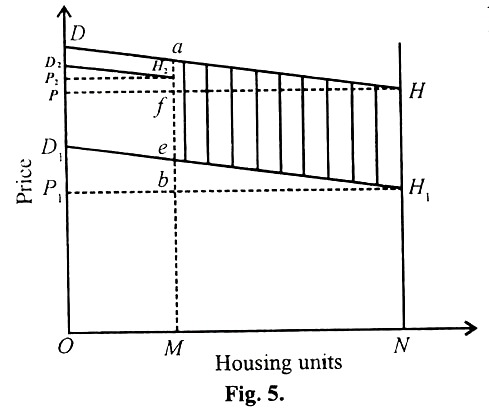
Now OM quite houses are more valuable so the demand curve shifts to D2H2. This position is fixed higher because people are willing to pay more for the quite houses. This is given by the distance ae=D. the distance between the demand curves DH and D1H1for marginal consumer of quite houses.
If this marginal willing to pay is not altered, the marginal consumer must be willing to pay P1 + D for quite houses. Hence adding D to P1 gives point H2 as the demand by the marginal consumer and similar analysis for other consumers gives the demand curve D2H2 as the demand curve for quite houses setting a price of P2.
According to the figure the observed house price differential after the introduction of noise concept is P2-P1 But the actual change in welfare is measured as the change in consumer surplus is given by the shaded area. This shaded area can be analyzed as
aHH1b = afH + feH1H-ebH1
Giving the symbol ‘S’ for consumers’ surplus, for the surplus at the original price P and Si for the surplus at the new price of the noisy house P1 this becomes.
^S = So + (P-P1) MA’ – Si (or) (P-P1) MN + (So-Si)
This reveals that the measure of welfare loss to the house price is the differential between the initial ‘no noise’ situation and the new price of noisy houses plus the change in surplus between the initial ‘no noise’ situation. But the formula we derived earlier stated the difference between the new price for quite houses and the new price for noisy prices. From the figure we can observe the following inequality.
(P-Pi) MN < S < (P2– P1) MN
This means, the approach using only the difference between the no-noise and noise situation will understate noise cost and an approach using the differential between the new price of noisy houses will overstate noise costs.
5. Merits and Demerits of Cost Benefit Analysis:
Merits:
(i) The cost benefit analysis may be applicable for both the new as well as old projects.
(ii) The cost benefit analysis is based of accepted social principle that is on individual preference.
(iii) This method encourages development for new techniques for the evaluation of social benefits.
Demerits:
(i) The government is not completely aware of all the costs and benefits associated with the programme.
(ii) This approach does not clearly state that who should bear the pollution control costs.
(iii) The method of collecting data for this analysis is generally biased.
(iv) The people will have different value system and there will always be loser in the process.