Economic Concepts: Top 10 Basic Economic Concepts – Discussed!

Read this article to learn about the ten basic economic concepts:

(1) Demand Curve Concepts in Monopolistic Competition, (2) Concepts of Marginal Product in Business Economics, (3) Narrower Concept of Growth in Economics, (4) Ricardo’s Concept of Terms of Trade and Reciprocal Demand, (5) Concept of Equilibrium, and Others.

Concept # 1. Demand Curve Concepts in Monopolistic Competition:

Monopolistic competition is an amalgam of perfect competition and monopoly. A monopolistically competitive firm does not face a horizontal demand curve. On the other hand, a competitive firm experiences horizontal demand curve since goods produced by all firms are homogeneous goods. Product differentiation, however, is one of the chief assumptions of monopolistic competition.

In this market, goods are not perfect substitutes like perfect competition. Goods produced by large number of monopolistic competitors are closely related to each other. Each product is a very close substitute of the product of others. It is due to this product differentiation that every firm enjoys some sort of monopoly power. Each product is unique. Then the demand curve faced by a monopolistically competitive firm is negative sloping.

For building up his model of monopolistic competition, Chamberlin considers two demand curves—proportional demand curve or actual- sales curve and perceived demand curve or anticipated demand curve. The former is drawn by assuming that all the monopolistically competitive firms charge the same price.

On the other hand, a perceived demand curve is drawn on the assumption that the competitor sellers will not change the original price. The curve D_P is the proportional demand curve. This is the demand curve faced by a particular firm when all the sellers charge the same price. D_A is the anticipated or perceived demand curve facing the firm if all sellers maintain the original price.

Let us start with a price of OP₁ and output sold OQ₁. Now if a typical firm wishes a cut in price from OP₁ he will expect his sales to go up. This is because Chamberlin assumes that all other firms will keep their prices at OP₁. Similarly, if the particular seller plans to raise the price of the product, he can expect a drastic drop in sales since all other sellers will keep their price at OP₁. Thus, the individual firm perceives a demand curve D_A at price OP₁ since every seller ‘expects his action to go unnoticed by his rivals’.

D_A curve is more elastic than D_P because each firm in this model believes that no other firms will react or respond to changes in its price change.

Anticipating elastic demand, each firm has an incentive to lower the price of its product in order to capture a larger share of the market. In other words, if a particular firm reduces price of its product from OP₁ to OP₂, it can expect its sales to increase to OQ₃. Since every firm hopes that no other firms will cut price, the gain in the ultimate analysis will be smaller. If all firms reduce price to OP₂, the actual sales will be OQ₂ instead of OQ₃. In view of this, D_P curve is more steep or less elastic than D_A curve.

D_P curve shows the actual sales since it takes into account the effects of the actions of competitor sellers to the price changes. On the other-hand, D_A curve shows anticipated changes in quantity sold when it contemplates a price change. Under this market form, every seller believes that his actions will go unnoticed. Thus, every firm ignores the reaction of rival sellers and, hence, behaves independently. All firms acting independently actually sell less than what they anticipate.

However, to make it simple, we have not used anticipated or perceived demand curve to describe equilibrium situation of a firm under monopolistic competition both in the short run and in the long run.

Concept # 2. Concepts of Marginal Product in Business Economics:

i. MPP:

MPP is the change in total product consequent upon a change in the use of an input. For the sake of analysis, we assume that our firm uses labour as a variable input and all other inputs are held constant. Thus, MPP of labour or symbolically MPP_L, is the change in total product (TP) due to a change in the use of labour, i.e.,

MPP_L = Change in total product/Change in number of labourer

Or MPP_L = ∆TP/∆L

ii. VMP:

When MPP is expressed in monetary terms we obtain VMP. If we multiply MPP by the price of the good, say X (P_x), we obtain money value of MPP;

VMP = MPP × P_X

Assuming labour as the variable input,

VMP_L = MPP_L × P_X

iii. MRP:

MRP is the change in total revenue resulting from the employment of additional unit of a variable input in question’. In other words, MRP of labour is the change in total revenue attributable to a change in the employment of labour, i.e.,

MPP_L = Change in total revenue/Change in number of labourer

or MPP_L = ∆TP/∆L

MRP may also be defined as MPP of the variable input multiplied by marginal revenue (MR). In terms of labour,

MRP_L = MPP_L × MR

Concept # 3. Narrower Concept of Growth in Economics:

Economic growth and economic development are not synonymous. Economic growth may be a necessary condition for economic development of countries, but it is not a sufficient condition.

In fact, economic growth does not give us correct assessment of an economy for the following reasons:

Per capita income growth does not measure welfare:

Firstly, economic growth is associated with an increase in GNP/GDP per capita. It measures wrongly—per head GNP does not, by Itself, constitute or measure of welfare or success in development. GDP assumes that people have money or assets and thus operate in the market without any hitch.

It is observed that a vast number of people fail to operate m the market as they don’t have enough money or assets and are subject to torture and exploitation by the people who have money or assets. This then suggests that per capita income does not give any information about income distribution. It is observed that, despite high rate of growth, some of the countries experience high incidence of poverty and unemployment.

Secondly, economic growth does not talk about the quality of life. Undernutrition, diseases, and the associated problems of lower life expectancy at birth and higher infant mortality rates, literacy rates, and many other indicators of health and education of different populations comprise human development. In poor developing countries (i.e., global South), people end themselves at low level of literacy, low standards of health and nutrition, etc. Miseries arising from lack of food and shelter do not get reflected in the concept of economic growth.

Rising per capita income gives us the impre­ssion that the economy is growing, wealthier. But it does not take into account the above-noted aspects of life. India’s GDP is rising but she is down in terms of other indicators. It has been revealed that 42.3 p.c. of under- 5 Indian children are severely and moderately underweight. This kind of undernutrition is a ‘national shame’. There is more to the ‘quality of life’ than having more income.

Growth ignores environmental issues:

Thirdly, economic growth does not deal with environmental issues. In the process of achieving higher economic growth, environmental considerations like deple­tion of renewable natural resources, air pollution, etc., are given little weightage. These aspects have an important bearing on the economic develop­ment of a country in the long run. Desire for higher and higher economic growth is associated with environmental damages. It is economic deve­lopment that cares for environmental issues.

Economic development ‘a multidimensional process’:

It is, thus, obvious that economic deve­lopment involves something more than economic growth. In fact, there are certain qualitative dimen­sions in the process of development that are cons­picuous by their absence in the growth or expansion of an economy. Economic development implies both more output and changes in the technical, institutional arrangements by which it is produced, and a change in attitudes and values.

“Development concerns not only man’s material needs but also improvement of the social conditions of his life. Development is, therefore, not only economic growth but growth plus change—social, cultural and institutional as well as economic. Development is, thus, not purely an economic phenomenon; it has to be conceived of as a multi-dimensional process.”

Naturally, economic development is a value-based concept. It should include not only the acceleration of economic growth but also the reduction of inequality and eradication of poverty, increase in employment opportunities and welfare of the masses, etc.

Growth is silent about the quality of life and broad human development:

However, economic development may mean more. Economic develop­ment must encompass human development. Amartya Sen defines economic development in terms of ‘entitlement’ and ‘capability’.

Entitlement refers to be set of alternative commodity bundles that an individual can command through the totality of rights and obliga­tions that he or she faces. Thus, ‘entitlements’ of people generate ‘capabilities’. Entitlements of people do not only depend on their incomes but also on a host of power relations in a society, the spatial distribution of resources in a society (like facilities of health care and schooling) and what individuals can accumulate from such supplied by the state. Capability represents a person’s freedom to achieve various functioning combinations. Thus, the notion of capability is essentially one of freedom—the range of options a person has in deciding what kind of life he or she wants to pursue.

Poverty, according to Amartya Sen, is a kind of ‘capability deprivation’. Sen says that economic development should be interpreted as a process of expansion of the freedoms that people enjoy. Important areas of unfreedom that people face are famine and undernourishment, mass illiteracy, poor state of health of people, lack of shelter and other basic needs, economic insecurity, denial of basic civil and political liberty, etc.

Through the policies of expansion of human capabilities, development processes can be initia­ted. That is why it is said that the basic objective of development is the process of expansion of entitlements and human capabilities. That is to say, how GNP growth is used to improve human capabilities and, in turn, how people utilise their capabilities is economic development.

Amartya Sen, thus, emphasises that, instead of concentrating on GNP or GDP, development economics should take into account both entitlements and capability expansion. He argues that income does not necessarily address the nature of entitlement. Taking a cue from the Chinese famine (1958-1961) as well as the Bengal famine (1943), he emphatically demonstrated that famines, in general, were to be attributed to the entitlement failure rather than the shortage of food. Despite abundant supplies in food, people had to suffer miserably from hunger and famine in Bengal due to the entitlement failure in collecting food from the market. Famine is one source of unfreedom.

Sen Says: “Development requires the removal of major sources of unfreedom.” The basic condi­tion for economic development are the freedoms from hunger and famine, malnutrition, deficient schooling, poverty, poor health, economic insecu­rity, denial of civil and political rights, social inequalities, etc. These human goals of economic development as emphasised by Amartya Sen have brought about a radical change in development thinking—at least since the 1970s.

Amartya Sen, carrying on his value-loaded development economics, talks on social justice.

He says that undernourishment of children, absence of opportunities of basic schooling, lack of entitlement of basic medical attention, particularly to the underprivileged of our society, etc., are nothing but social injustices. Since most of these facilities—meant for all Indians—crowd out the underdogs through the dominant class or partners of the society, injustices pile upon the vulnerable sections of the population. This kind of gross injustice is nothing but denial of development or ‘exclusive development’. Thus, in the development discourse, social justice—a more normative concept—needs to be provided to all. And that is economic development.

How economic growth and economic development are interrelated can be known from the Fig. 1.1.

Growth says nothing about Gross National Happiness (GNH):

With the change in development thinking ‘new’ measures of success have been unveiled—social well-being is an important component of development. In other words, well-being has emerged as a substitute for ‘wealth’. Overall public happiness or satisfaction with life describes well-being. The GNH aims to ensure that prosperity or well-being is shared across society and it is balanced against preserving cultural identities and traditions, protecting the ecology, preserving democracy with social equality.

We have seen that ‘growth is not necessarily good’ as it ignores some very crucial issues. Growth does not increase human well-being. Growth may improve standard of living but undermines ‘quality of life’. That why, today, we see ‘de-growth’ movement—a movement that attempts to shift emphasis from material goods to non-material factors, or human well-being or, more specifically, ‘happiness’.

Economic progress of a country is to be measured not only in terms of GNP/GDP or poverty-unemployment-inequality but also in terms of ‘pursuit of happiness’. Economic progress must be such that happiness levels of people across society without damaging environment need to be included. Happiness of people is measured through surveys when people are asked to assess how happy they are. This ‘happiness index’ is used in Bhutan—the Buddhist economy— and is called ‘Gross National Happiness’ (GNH), National happiness score is attained when basic needs of the people are met. These are: housing, wealth, employment, environment protection, peaceful atmosphere, morality, basic healthcare, presentation of cultural traditions, love and respect, democracy, etc.

These aspects of life are missing both from the concepts of growth and even from economic development. Anyway, the economy does not grow in a conventional sense. GNH uses more complex hybrid indicators. Some of these elements are invisible things but essential to our happiness or well-being.

As per 2007 GNH criterion, Bhutan was ranked the second fastest developing country in 2007. To keep the level of happiness of Bhutanese people, a decree had been issued for affores­tation of the country to the extent of 60 p.c. But, since tourism has the potentiality of damaging environment, it has also been decided that it needs to be controlled and regulated. Otherwise, tourism will pull down the level of GNH. Thus the end of happiness depends on how environmental damages are minimised.

Till the other day, we had been concentrating more on the wrong indicator—the GNP/GDP— for too long. However, measurement of ‘GNH’ is a difficult task. Anyway, the concept of GNH is gaining ground—Canada, France, Costa Rica, U. K. and many other countries have been contemplating on measuring GNH. The basic objective is to measure ‘social welfare’.

Concept # 4. Ricardo’s Concept of Terms of Trade and Reciprocal Demand:

Specialisation and exchange benefit all the trading partners. Because of complete specialisation in the production of the commodities in which countries have comparative advantages— as suggested by Ricardo, global production becomes larger. Now, if every country trades with each other, every country will gain from such exchanges.

However, such gain from specialisation and exchange depends on the terms of trade (TOT). It refers to the quantity of imports that exports buy. It is measured by the ratio of export price to import price. It is the ratio at which a country can export or sell domestic goods for imported goods.

Let P_x be the price of export good and P_m be the price of import good. Thus, the (barter or commodity) TOT are defined as P_x /P_m

In the real world, where countries export and import a large number of goods, TOT are computed as an index number:

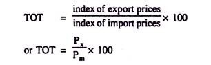
To calculate the index of export and import prices, we choose a base year and the current period. A base period index of export and import price is 100. Thus, TOT for the base year is 100. Suppose export price index rises to 120 and import price index rises to 110. Thus,

Tot rise to 109. This means that a unit of exports will buy 9 p.c. more imports than the old TOT. TOT thus improves. A fall in the TOT, on the other hand, implies unfavourable TOT in the sense that the country concerned will now use more exports to buy the same quantity of imports.

On .which factors the TOT depend? Answer to this question was unknown to Ricardo. In other words, Ricardo could not locate the exact TOT at which trade takes place. This is because of the fact that Ricardo concentrated on the cost or the supply side of production and ignored demand conditions. Anyway, Ricardo suggested that the TOT would settle in-between two domestic cost ratios. We explain first the Ricardian notion of TOT and then Mill’s concept of reciprocal demand.

Let us assume that the internal or domestic cost ratio in country A is 1 X for 1.5 Y, and, in country B, it is 1 X for 2 Y. This domestic cost ratio suggests that country A has a comparative advantage in X while country B has a comparative advantage in Y. Thus, A and B will trade with each other. But what would be the TOT at which both will trade? Ricardo argued that international TOT would lie somewhere between 1: 1.5 and 1: 2 and both the countries would stand to gain.

It was J. S. Mill who successfully determined the exact TOT by introducing the concept of reciprocal demand. In other words, actual TOT depends on the relative prices of X and Y after trade takes place. Or TOT depends upon the strength of the world supply and demand for each of these two commodities.

This is what Mill called reciprocal demand. These relative prices will depend upon the strength and elasticity of each country’s demand for the other country’s product or upon reciprocal demand. If the TOT lie very close to 1: 1.5, then country A would gain very little and she would not offer much X for export.

However, at this TOT, country B would gain quite a large amount since it would demand more X by offering less Y. Consequently, country B’s demand for imports of X would exceed country A’s supply of exports of X, and so the price of X in terms of Y would rise.

As the TOT rises to 1 : 1.6; 1 : 1.7, etc., country A offers more X to buy more Y, while country B demands less Y to buy X. In this way, a particular TOT would prevail at which the value of each country’s export equals its value of imports. In this way, reciprocal demand is equated in the two countries at the international TOT.

Thus, TOT lies between the upper and lower limits of domestic cost ratios of the two countries. Equilibrium or international TOT brings equality between export and import. At the equilibrium TOT world output equals world consumption. But the gains to both the countries need to be equal. However, more favourable the TOT to any country, greater is the welfare of a country. A tariff imposed on importable may, however, bring TOT in favour of the tariff-imposing country. However, if the tariff rate exceeds the optimum tariff rate, gains from trade may reduce even though TOT may be favourable. Thus, a favourable TOT does not necessarily increase welfare of a nation. Still then, TOT must not be adverse.

Concept # 5. Concept of Equilibrium:

Equilibrium is a concept borrowed from mechanics where we get the idea of equilibrium system of forces. In mechanics a system of forces is said to be in equilibrium if two forces making to move the body in opposite directions are counter-balanced. Thus, an equilibrium situation is a state of rest.

In economics we use the term to mean that a single price for a product is established in a market and when no economic forces are being set up to change that price. In other words, in equilibrium, the price and quantity of a commodity match both consumers’ and producers’ expectations and thus there is no discrepancy between the actual and desired prices and quantities.

Consequently, market is cleared and there are no involuntary holdings of unsold stocks. The equilibrium behaviours of consumers and producers — whether in a single market or in the economy as a whole — is characterised by the fact that there exists no feeling of urgency on the part of the buyers and sellers to change their behaviour.

In contrast, disequilibrium situation is one in which some buyers and sellers feel compelled to change their behaviour because forces are at work that change their circumstances. By changing their behaviour, however, they change the circumstances of other producers and consumers who may initially have been in equilibrium. A disequilibrium sets in motion a chain of adjustment and readjustment processes; for example, on the stock market, buyers and sellers change their behaviour daily in response to changing circumstances.

The economy as a whole would be in equilibrium when the planned demand for output is equal to planned supply of output. The whole economy would be in equilibrium when aggregate demand equals aggregate supply.

Equilibrium analyses are of two types: partial equilibrium and general equilibrium. In partial equilibrium analysis equilibrium is reached in one market assuming that all other things remain unchanged. However, in general equi­librium analysis, different markets of the economy are interdependent. In microeconomics, partial equilibrium analysis is generally used. But, in macroeconomics, general equilibrium analysis is usually used as in the classical or the Keynesian macroeconomic systems.

An equilibrium is a state of rest in which no economic forces are being generated to change the situation. In a market for a good, such a state of rest can be said to exist when there is neither excess demand for nor excess supply of the good.

An equilibrium is said to be a stable equilibrium when economic forces lend to push the market towards it, or any divergence from the equilibrium position generates forces which tend to restore the equilibrium. However, the equilibrium could be unstable when a small change in equilibrium price sends the system further and further away from equilibrium.

Concept # 6. The Incremental Concept:

It is easy to describe incremental reasoning. But it is very difficult to apply it. As T.J. Coyne has put it, “It involves estimating the impact of decision alternatives on costs and revenues, stressing the changes in total cost and total revenue that result from changes in prices, products, procedures, invest­ments or whatever may be at stake in the decision”. Two basic concepts lie at the heart of incremental analysis, viz., incremental cost and incremental revenue. The former refers to the change in total cost resulting from a decision. Likewise, the latter may be defined as the change in total revenue re­sulting from a decision.

A decision is surely profita­ble if:

1. It increases revenues more than it increases cost.

2. It reduces some cost more than it increases oth­ers.

3. It increases some revenues more than it de­creases others.

4. It decreases costs more than it decreases reve­nue.

We may now consider some of the implications of incremental reasoning which appears to be too elementary. In general, businessmen think that in order to make an overall profit they must make a profit on every activity (or job). Consequently they refuse orders that do not cover cost (labour, materi­als and overhead) and make a provision for profit. This is an unproved and probably a false belief. In­cremental reasoning makes it clear that this rule may be inconsistent with short-rim profit maximi­zation.

A refusal to accept a job below cost may im­ply rejection of a possibility of adding more to reve­nue than to cost. Here the relevant cost for decision-making is not the full cost but rather the incremen­tal cost. The following example clarifies the point. Consider a new order which is supposed to bring Rs. 9,000 additional revenue.

The costs are estimat­ed as follows:

It apparently seems that the order is unprofita­ble. But suppose there is idle capacity in the short run. This could be used to produce the order. Sup­pose acceptance of the order will add only Rs. 900 of overhead. Suppose neither extra selling cost nor extra administration cost is involved in the order. Moreover, only part of the labour cost is incre­mental, since permanent workers; who are sitting idle, may be put to work without extra pay.

Suppose the incremental cost of accepting the order is as follows:

Although at first sight it appeared that the or­der would results in a loss of Rs. 1200, it is now clear that it will bring an additional profit of Rs. 2,800. However, incremental reasoning does not mean that the firm should fix the price at incremental cost or should accept all orders that just cover incre­mental costs. True, ‘charging what the market will bear’ is quite consistent with instrumentalism, for it implies raising prices as long as the resulting reve­nues increase.

In our example, the acceptance of the Rs. 9,000 order is based on assumption that there is idle capacity which could be fruitfully utilized to execute the order. It is also implicitly assumed that there is no other profitable alternative. If there is a more profitable alternative, it has to be accepted.

So the essence of the incremental principle is that: a decision is to be considered as sound and ra­tional if it increases revenue more than it increases cost, or reduces cost more than it reduces revenue.

Marginalism:

Incremental reasoning is closely related to two important concepts of traditional ec­onomics, viz., cost and marginal revenue. However, there are similarities and differences.

The follow­ing two points may be noted in this context:

1. Marginal cost and revenue are always defined in terms of unit changes in output, but incremental cost and revenue are not necessarily restricted to unit changes. Usually marginal cost is expressed as the ratio of two absolute changes, viz., change in total cost and change in output, i.e., MC = dC/dQ. Likewise MR = dTR/dQ where MR is marginal rev­enue and TR is total revenue.

A simple example will illustrate the two con­cepts: the marginal concept and the incremental concept. Suppose, the extra cost of producing one ex­tra unit of output is Rs. 10 and the extra revenue made by selling this extra unit is Rs. 15. If a 5-unit increase in output increases total cost by say Rs. 45 (from say Rs. 350 to Rs. 395), and increases revenue by Rs. 70 (from say Rs. 400 to 470), we can speak of an incremental cost of Rs. 45 and an incremental revenue of Rs. 70. In this case the unit (average) MC over this range of output is Rs. 9 and unit (average) MR is Rs. 14.

2. Incremental concepts are more flexible than marginal concepts. In general we restrict the two terms: MC and MR to the effects of changes in out­put. But managerial decision making is not to be concerned with changed output at all. For example, the production manager may be faced with the problem of substituting one process of production (or activity) for another to produce the same output.

The problem here is one of comparing the cost of the first process with -that of the alternative. Marginal analysis is not suited for this type of de­cision. It is, of course, possible to compare the MC of one process with that of another but not of the MC of the change. However, the term ‘incremental cost’ may be used to refer to the change in cost brought about by the changes in production process or activity.

The following diagram may be used to compare the marginal and incremental approaches: 

In Fig 1.1 the MC curve is rising over most of its range.

Suppose the production manager is considering an increase in output from 2,000 to 3,000 units. In this case it is very difficult to measure the marginal cost of change. No single MC cost figure will suffice. The MC is initially low, but subsequently it rises rapidly.

However, another pattern of costs is common in industry. Several empirical studies have discov­ered relatively constant marginal costs over wide range of outputs, as in Fig 1.2. Here MC does not change dramatically with the changes in output. Hence a single MC cost figure can be used over the whole range.

For the firm illustrated in Fig 1.2, we assume that total fixed cost is Rs. 4,000 per unit of time. The aver­age variable cost is Rs. 2.50 per unit. The MC is also Rs. 2.50 per unit. Suppose, the production manager has to choose between an output of 2,000 units and one of 3,000 units. In this case MC is Rs. 250 but incremen­tal cost is Rs. 2,500.

The pertinent question here is whether or not marginal costs are in fact constant and justify the substitution of incremental cost measurements over large changes in output, for measurements of cost changes for small (marginal) changes in output. If the short run cost curves were linear throughout, the decision-making problem would be greatly simpli­fied.

Concept # 7. The Concept of Time Perspective:

In economics, we often draw a distinction be­tween the short-run and the long-run. This distinc­tion is not based on any calendar period, say, a month, a quarter or a year. It is based in the speed with which decisions can be made and factors of production varied.

The period during which it is possible to vary some factors and not others is called the short run. But the period during which all factors can be varied is called the long-run. For example, more output can be produced in the short- run by using more labour and raw materials. This is basically a short-term decision. But setting up a new factory or building an entirely new plant is a long-term decision.

In reality, however, the distinction between the two often gets blurred. What remains is an estimate of those costs that vary and those that do not by the decision under consideration. In managerial economics we are concerned with the short-run and long-run effects of decisions on revenues as well as on costs. The line between the short-run and long-run revenue (or demand) is even less transparent than that for costs. What is really important for managerial decision making is main­taining the right balance among various runs, i.e., the long-run, short-run and intermediate-run per­spectives.

A decision may be made on the basis of certain short-term considerations but it may have various long-term repercussions which, in turn, may make it more or less profitable than it appeared at the first sight. A simple example will make this point clear. Suppose there is a firm with temporary idle ca­pacity. It now gets an order for 10,000 units. The prospective customer is willing to pay Rs. 3 per unit, or Rs. 30,000 for the whole lot. The short-term incremental cost (which ignores the fixed cost is) is only Rs. 2.50. So the contribution to overhead and profit is 50 paise per unit (or Rs. 5,000 in all).

But the following two long-term repercussions must be taken into account:

1. If the management commits itself to a series of repeat orders at the same price, the fixed costs (which are ignored temporarily) will become vari­able cost. For instance, sooner or later it will be­come necessary to replace the machinery and equipment which wear out. True enough, the grad­ual accumulation of orders may require an addition to capacity, with added depreciation and added top-level supervision.

2. If lower price is charged for the extra order, old customers who pay higher price for the same product may become annoyed. This practice will appear to be unethical and may destroy the compa­ny image. This will be damaging in the long-run.

Now on the basis of our above discussion we can state the above principle — the principle of time perspective — in the following words:

A decision should always take into considera­tion both the short-term and long-term effects on revenues and costs, giving proper weight to the most relevant time periods.

However, the real problem is how to apply this principle in specific situations to arrive at a deci­sion.

An example:

A large reputed printing company in Calcutta maintains a policy of never quoting be­low full cost even if it has some idle capacity. Al­though incremental cost is far below full cost, man­agement has found that the long-run repercussions of going below full cost more than offset any short- run gain.

Prima facie, price reduction for some cus­tomers would have an undesirable effect on cus­tomer goodwill, especially among regular custom­ers who will not benefit from rate reductions. Secondly, if the availability of idle capacity is unpredictable, there may be pressure on capacity when demand is high.

In fact when the order be­comes firm the situation might change, causing low-price orders to interfere with regular price business. Management would like to avoid this sit­uation. Otherwise, it would be considered as a firm that exploits the market when demand is unfavorable and allows price concessions when de­mand is favourable. This simple illustration re­veals the need to consider both the long-term and short-term impact of price policy.

Concept # 8. The Opportunity Cost Concept:

The opportunity cost of a decision means sacri­ficing alternatives. Opportunity cost measures the value of the most valuable of the options that we have to forego in choosing from a set of alternative options. Suppose a shipbuilder gets a contract to be called Contract A. After making the correct assess­ment of the associated incremental costs and reve­nues he arrives at an estimated profit of Rs. 25,000 from the contract. Suppose, in the meantime, two other contracts, B and C, have been brought to his attention.

These two are expected to give a profit of Rs. 15,000 and Rs. 20,000, respectively. However, his yard’s capacity is so limited that he can accept only one of these. So, in the absence of any other consideration, he would accept contract A, the most profitable one. His opportunity cost would then be Rs. 20,000, the sacrifice he must make of the profit for the next best option. Had he chosen either B or C, his opportunity cost would have been Rs. 25,000 profit that A would have earned.

An opportunity cost has arisen here only because some essential input, the yard’s capacity, is scarce, i.e., grossly insufficient to take up all the options that are open and desirable. In the absence of such a constraint no such sacrifice and hence no opportu­nity cost would have arisen. We will come across various examples of opportunity cost in this title because all business activity is carried on within constraint (‘scarcities’) which force choices and consequent sacrifices to be made.

The following examples help in understanding the meaning of the term:

1. The opportunity cost (O.C.) of using a ma­chine is the most profitable alternative sacrificed by employing the machine in its present use.

2. The O.C. of buying a colour TV is the interest or profit that could be earned by investing the pur­chase money.

3. The O.C. of working for oneself in one’s own factory is the salary that one could earn in others occupations.

4. The O.C. of funds tied in one’s own business is the interest (or profits adjusted for difference in risk) that could be earned on those funds in other ventures.

However, if machine has been lying idle for some time, the O.C. of bringing it into production is nil. Similarly the O.C. of using idle space is obvi­ously less than that of using space needed for other activities. So O.C.s require the measurement of sacrifices, real or monetary. If a decision involves no sacrific­es, it is cost free. The expenditure of cash (for raw- materials, say) involves a sacrifice of other possi­ble expenditures and is therefore an O.C. Thus the only costs for decision-making are opportunity costs.

However, all O.C.s do not involve actual mone­tary payments. A man in a desert or in a distant is­land (like Robinson Crusoe) might have the choice between picking coconuts or fishing. The O.C. of co­conuts is the amount of fish that might be obtained with the same amount of time and effort — irre­spective of how much the man likes shinning up trees.

O.C.s are important when considering make-or- buy decisions, as also when deciding whether or not to sell. For instance, the alternative to using busi­ness premises which one owns as offices is to rent or sell them. The O.C.s is the rental forgone, or the difference between the expected market value at the beginning and end of the year, whichever is higher.

One form of opportunity cost which is likely to be used is in the analysis of capital projects. The discount rate used to find out net present values when evaluating capital projects is nothing but an opportunity cost of capital. The alternative to car­rying .out the project is to invest the money in a safe alternative and the evaluation is designed to ascertain whether the project yields a higher re­turn. This concept of O.C. is discussed in the context of capital expenditure decisions later.

Closely related to our above discussion is a dis­tinction between explicit and implicit costs. Explic­it costs are those that are reflected in the book of accounts, such as payments for raw-materials and labour. On the contrary, implicit (or imputed) costs are those sacrifices (such as the interest on the owner’s own investment) which are not reflected in accounts. Some writers equate O.C.s with implicit costs. The truth is that O.C.s cover all sacrifices, implicit or explicit.

In reality, however, some explicit expenses may not involve sacrifices of alternatives. For example, a company like Texmaco Ltd. paid wages to idle la­bour in periods of slack activity. These wages were in the nature of a fixed cost and were not included in the O.C. in a decision to use that labour in some other activity.

From the above discussion we can derive anoth­er principle — the O.C. principle — as follows:

The cost involved in any decision is the sacrific­es of alternatives required by that decision. In case there is no sacrifice, there is no cost either.

Large firms often make uses of the O.C. concept. They use linear programming models, replacement models and other optimization techniques. These are all based on the O.C. concept.

Concept # 9. The Contribution Concept:

Consider a simple product whose price is deter­mined either by the market forces the forces of demand and supply, or by some government agency like the Bureau of Costs and Industrial Prices (Govt, of India, New Delhi). Assume this price is Rs. 93. The total cost including allocated over­heads is Rs. 105, but the incremental cost is only Rs. 74. The loss on the item seems to be Rs. 12. So at first sight the firm may think of dropping the product. However, if the contribution to overhead and profits is Rs. 19 = (Rs. 93 – Rs. 74), further anal­ysis is required before arriving at a decision.

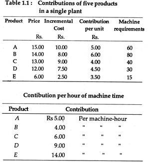
It is not always worthwhile to retain a product simply because its contribution is positive. If the company is having a package of orders on products (say, B, C or D) requiring the same scarce resources per unit — production time or machine time and la­bour — and if these products make larger contribu­tions, viz., Rs. 50 or Rs. 40 or Rs. 30, there is no point in sacrificing these larger contribution in favour of product A. However, what is important is the com­parison of contributions, not the comparison of prof­its or losses based on full costs.

Suppose the only production constraint in a multi-product firm is machine-hours available. Now we can convert the contribution per unit of output into contributions per machine-hour. Table 1.1 il­lustrates such a situation in case of a company pro­ducing five products.

At first sight product B appears to be the best. Since its contribution is the highest, it deserves the top priority in allocation of capacity. But product B’s demand on capacity is also maximum. By con­verting the contributions into contributions per hour of machine time, we get the following results.

Now it is clear that the product E, which ini­tially appeared to be the least profitable, is now the largest contributor. Therefore, the principle should be almost the opposite to those that ap­peared at first glance. If there are more constraints, i.e., more than one capacity bottleneck and all products pass through, say, four or five different processes, it will no long­er be possible to compute contributions in terms of one of the bottlenecks. We have to make use of lin­ear programming to reach an optimum solution (i.e., to choose an optimum product mix).

So long we assumed that demand for each prod­uct remained unchanged as also its price. Now sup­pose the quantity demanded of product E increases at a lower price. Now we can compare product E’s contribution of Rs. 2.50 at a price of Rs. 6 with its contribution of Rs. 3 at a price of Rs. 5.50.

If sales at a higher price are 8,000 units and at the lower pric­es 15,000 units, the total contribution from product E increases from Rs. 28,000 to Rs. 45,000. So, it is in the Tightness of things to accept the lower unit con­tribution to obtain the higher volume, even if other higher unit contribution products are sacrificed.

The contribution concept is often used in product- mix decisions, also in pricing decisions. It is also applicable in make or buy decisions. Finally, in a discussion on capital budgeting, it is usually discov­ered that the cash flows estimated by financial analysis are closely related to the contribution con­cept.

Concept # 10. T.J. Coyne’s Concept of Reasonable Profit:

The amount called profit on a firm’s profit and loss statement is usually much larger than the eco­nomic profit of the firm. As T. J. Coyne has pointed out, “To determine economic profit, a competitive or normal rate of payment for services of capital sup­plied by the firm must be subtracted from the profit for the period determined by conventional account­ing methods.

This capital supplied by the firm is the market value of land, plant, equipment, working capital and the net amounts borrowed against the physical assets.” The concept of reasonable profit is none other than the normal or going rate of return on capital supplied by the firm. It is also called the opportunity cost of capital and is a part of business cost, or a part of the economic profit.

Economists often draw a distinction between net profit and normal profit. The concept of reason­able profit is illustrated by the term “normal profit”. It is assumed in economic theory that where compe­tition among entrepreneurs is perfect, the price of a product is equal to average cost which includes ‘nor­mal profit’.

The implication is clear: no one can stay in the business if the price he gets is what he paid to make his product. Some economists have spoken of the element called the ‘wages of superintendence’ and suggested that the entrepreneur will want this as his minimum reward, or take his services else­where (where return is supposedly higher). This concept is questionable, and in any case the amount of this reward is vague. So is ‘normal profit’. All one can do is to regard it as what the ‘average’ undertak­ing in this line of business, conducted with average ability, is getting as profit.

The profits formula is simply expressed as:

Profits = Total revenue—total costs i.e.,

π = TR – TC.

The total revenue portion of this formula is de­fined similarly by both groups. Thus the differences in profit measurement stem from disagreements in the measurement of total cost.

From the perspective of an accountant, the only costs (with the exception of depreciation) that are relevant are the explicit costs of doing business dur­ing an accounting period. These explicit costs are recorded in the accounting statements and are based on the actual or outlay cost during a particular time period.

To an economist, these explicit costs are only the starting point in measuring all of the costs, as­sociated with conducting affairs within a business enterprise. Recall that opportunity cost refers to the cost associated with the next best opinion or alterna­tive that is lost or foregone.

The four major factors used by a firm are labour, land, capital and organisa­tion (or entrepreneurship). Since these resources are scarce, their utilization in any given activity involves a real cost.

Whether or not this cost is included in the accounting records is irrelevant when attempting to obtain a complete measure of opportunity cost. Thus, it is clear that the economist’s view of cost includes both the explicit costs as measured by the accountant, and the implicit costs of using resources supplied by the owner manager.

Both the accountant and the economist agree that depreciation is an implicit cost of production, but economists would question the use of rapid de­preciation over a three-year period when there is hardly any logical basis for this accelerated depre­ciation, which leads to an understatement of profits on the accounting statement.

There are three general areas of implicit cost that are of importance to the economist:

1. The entrepreneur’s wages;

2. Rental income on land used in the business;

3. A normal rate of return for the capital invested by the owner.

To illustrate how these costs are computed let us consider an individual who currently earns Rs. 40,000 a year and has saved Rs. 20,000. This in­dividual is trying to decide whether to remain in his current salaried job and leaving his savings in an account that is yielding 10%, or to open his own business.

In order for it to be economically prof­itable to open his own business, not only must all explicit or accounting costs be covered but he must also earn enough to cover his forgone salary of Rs. 40,000 (ignoring any nonmonetary benefits associ­ated with being his own boss). If he uses the Rs. 20,000 as start-up equity, he is giving up the oppor­tunity to earn the interest on Rs. 20,000 he has saved.

From an economic point of view, the forgone salary and interest are genuine implicit costs of the new business. It is so because if the individual does not earn this minimum sum above explicit costs, he will find it more gainful to work for someone else and to invest his savings in some other alternative.

Thus, cost in the economic sense refer to transfer costs for opportunity earnings, i.e., to all payment necessary to keep resources employed in their current alterna­tive. If total revenue just equals total costs, this zero level of profit is referred to as normal profit. In fact, normal profit is the minimum supply price of entrepreneurship. It is the minimum sum that must be paid to the entrepreneur to carry on his present busi­ness. To the extent that TR exceeds TC, abnormal or economic profits are earned. Thus, to reconcile accounting and economic profits, all excluded im­plicit costs must be deducted from accounting profit (alternatively, added to explicit costs).

However, it is difficult to make a distinction be­tween normal and economic profits in practice, but the two measures perform entirely different func­tions. Normal profits are the compensation neces­sary to keep the resources employed in their present activities whereas economic profits are the market signals for expansion or contraction.

To the extent that accounting profit overstates (due to exclusion of implicit costs) or understates (due to inflated de­preciation allowances) economic profits, it provides incorrect signals to entrepreneurs, investors, and fi­nancial institutions.

Profits in Practice:

In economics profits are generally defined as the excess of total revenue of an enterprise over its total costs.

In economic theory profits are assumed to be the return to ownership of capital and the return to entrepreneurship. In a simple organization, where ownership and entrepreneurship coincide, it is very easy to measure profit.

However, in most large and complex organisations there is separation of owner­ship from control. Capital is extensively borrowed and most shareholders have little to do with com­pany management or entrepreneurship. Therefore, it is difficult to identify separate returns to owner­ship, management, and entrepreneurship in practice.

In the words of R. Eisner, “Where capital is partly owned and partly borrowed, accounting con­ventions denote a return to borrowed capital as in­terest, while including the return to the owned capi­tal as profit. Where owners work in managing their firms, the value of their labour or managerial ser­vices is usually included in profit, except to the ex­tent that owners formally pay themselves salaries.”