Choice Under Uncertainty (With Diagram)

Read this article to learn about Choice Under Uncertainty:- 1. Subject-matter of choice under uncertainty 2. Describing risk of choice under uncertainty 3. Preference towards Risk 4. Different Preferences towards Risk 5. Reducing Risk 6. Diversification 7. Insurance 8. Value of Information 9. Demand for Risky Assets 10. Assets and other things.

Choice under Uncertainty # 1. Subject-Matter:

Many of the choices that people make involve considerable uncertainty.

Sometimes we need to choose between risky ventures.

For example, what should we do with our savings? Should we invest in something safe, such as a bank savings account, or something riskier but more lucrative, such as the stock markets? Another example is the choice of a job or a career.

Is it better to work for a large, stable company where job security is good but the chances of advancement are limited, or to join a new venture, which offers less job security but quicker advancement?

To answer these questions, we must be able to quantify risk so as to be able to compare the riskiness and alternative choices.

Next, we will see how people can deal with risk or reduce risk — by diversification, by buying insurance, etc. or by investing in additional information. In different situations, people must choose the amount of risk they wish to bear. To analyse risk quantitatively, we need to know all possible outcomes of a particular action and the likelihood that each outcome will occur.

Choice under Uncertainty # 2. Describing Risk:

Probability:

Probability refers to the likelihood that an outcome will occur. Suppose the probability that the oil exploration project is successful might be 1/4, and the probability that it is unsuccessful 3/4. Probability could be objective and subjective. Objective probability relies on the frequency with which certain events have occurred.

Suppose we know from our experience that, of the last 100 offshore oil explorations, 1/4 have succeeded and 3/4 have failed. Then the probability of success of 1/4 is objective because it is based on the frequency of similar experiences.

But what if there are no similar past experiences to help measure probability? In these cases, objective measures of probability cannot be obtained, and a more subjective measure is needed. Subjective probability is the perception that an outcome will occur and the perception is based on a person’s judgment or experience, but not on the frequency of outcome observed in the past.

Whatever be the interpretation of probability, it is used to calculate two important measures that help us describe and compare risky choices. One measure tells us the expected value and the other variability of the possible outcomes.

Expected Value:

The expected value of an uncertain event is a weighted average of the values associated with all possible outcomes, with the probabilities of each outcome used as weights. The expected value measures the central tendency. Suppose we are considering an investment proposal in an offshore oil company with two possible outcomes: success yields a payoff of £40 per share, while failure yields a payoff of £20 per share.

The expected value in this case is given by:

Expected Value = Pr (success) (£40/share) + Pr (failure) (£20/share)

= 1/4 (£40/share) + 3/4 (£20/share) = £25/share.

More generally, if there are two possible outcomes having pay offs X₁ and X₂, and the probabilities of each outcome are given by Pr and Pr₂, then the expected value E(X) is: E (X) = Pr₁X₁ + Pr₁ X₂ ………….. (1)

Variability:

Suppose we are choosing between two sales jobs that have the same expected income (£1,500). The first is based on commission. The second job is salaried. There are two equally likely incomes under the first job — £2,000 for a good sales effort and £1,000 for a moderate effort. The second job pays £ 1510 most of the time, but would pay £510 in severance pay if the business goes burst.

Table 5.1 summarizes these possibilities:

The two jobs have the same expected income because .5 (£2,000) + .5 (£1,000) = .99 (£1,510) + 0.1 (£510) = £1,500. But the variability of the possible payoffs is different for the two jobs. The variability can be analysed by a measure that presumes that large differences between actual payoffs and the expected payoff, called deviations, signal greater risk.

Table 5.2 gives the deviations of actual incomes from the expected income for the two sales jobs:

In the first job, the average deviation is £500:

Thus,

Average Deviation = .5 (£500) + .5 (£500) = £500

For the second job, the average deviation is calculated as:

Average Deviation = .99 (£10) + .01 (£990) = £19.80

The first job is, thus, substantially more risky than the second as the average deviation of £500 is much greater than the average deviation of £19.80 for the second job. The variability can be measured either by the variance which is the average of the squares of the deviations of the payoffs associated with each outcome from their expected value or by the standard deviation (σ²) which is the square root of the variance.

The average of the squared deviations under job 1 is given by:

Variance (σ²) = .5 (£2, 50,000) + .5 (£2, 50,000) = £2, 50,000

The standard deviation is equal to the square root of £2, 50,000 or £500.

Similarly, the average of the squared deviations under Job 2 is given by:

Variance (σ²) = .99 (£100) + .01 (£9, 80,100) = £9,900.

The standard deviation (a) is the square root of £9,900 or £99.50. We use variance or standard deviation to measure risk, the second job is less risky than the first. Both the variance and the standard deviation of the incomes earned are lower. The concept of variance applies equally well when there are many outcomes rather than just two.

Decision-making:

Suppose we are choosing between the two sales jobs described above. What job should we take? If we dislike risk; we will take the second job. It offers the same expected return as the first but with less risk. Now suppose we add £100 to each of the payoffs in the first job, so that the expected payoff increases from £1,500 to £1,600.

The jobs can then be described as:

Job 1: Expected Income = £1,600 Variance = £2, 50,000

Job 2: Expected Income = £1,500 Variance = £ 9,900

Job 1 offers a higher expected income but is substantially riskier than job 2. Which job is preferred depends on us. If we are risk-lovers, we may opt for the higher expected income and higher variance, but a risk-averse person might opt for the second. We need to develop a consumer theory to see how people might decide between incomes that differ in both expected value and in riskiness.

Choice under Uncertainty # 3. Preference towards Risk:

We use the above job example to describe how people might evaluate risky outcomes, but the principles apply equally well to other choices. Here we concentrate on consumer choices generally, and on the utility that consumers derive from choosing among risky alternatives.

To simplify matters, we will consider the consumption of a single commodity, say, the consumer’s income. We assume that consumers know probabilities and that payoffs are now measured in terms of utility rather than money.

Fig. 5.1(a) shows how we can describe one’s preferences towards risk. The curve OB gives one’s utility function, tells us the level of utility that one can attain for each level of income. The level of utility increases from 10 to 16 to 18 as income increases from £10,000 to £20,000 to £30,000.

However, the marginal utility diminishes from 10 when income increases from 0 to £10,000, to 6 when income increases from £10,000 to £20,000, to 2 when income increases from £20,000 to £30,000.

Now, suppose, we have an income of £15,000 and are considering a new but risky job that will either double our income to £30,000 or cause it to fall to £10,000. Each has a probability of 0.5. As Fig. 5.1(a) shows, the utility level associated with an income of £10,000 is 10 (point A), and the utility level associated with a level of £30,000 is 18 (point B). The risky job must be compared with the current job, for which utility is 13 (point C).

To evaluate the new job, we can calculate the expected value of the resulting income. Because we are measuring value in terms of utility, we must calculate the expected utility we can get. The expected utility is the sum of the utilities associated with all possible outcomes, weighed by the probability that each outcome will occur.

In this case, expected utility is E(U) = 1/2U (£10,000) + 1/2U (£30,000) = 0.5 (10) + 0.5 (18) = 14.

The new risky job is, thus, preferred to the old job because the expected utility of 14 is greater than the original utility of 13. The old job involved no risk — it guaranteed an income of £15,000 and a utility level of 13. The new job is risky, but it offers the prospect of both a higher expected income and a higher expected utility of 14. If we wished to increase our expected utility, we would take the risky job.

Choice under Uncertainty # 4. Different Preferences towards Risk:

People differ in their willingness to bear risk. Some are risk-averse, some risk-lovers and some risk-neutral. A person who prefers a certain given income to a-risky job with the same expected income is known as risk-averse which is the most common attitude towards risk.

Most people not only insure against risks — such as, life insurance, health insurance, car insurance, etc. but also seek occupation with relatively stable wages.

Figure 5.1(a) applies to a person who is risk-averse. Suppose a person can have a certain income of £20,000 or a job yielding an income of £30,000 with probability 1/2 and an income of £10,000 with probability 1/2. As we have seen, the expected utility of the uncertain income is 14, an average of the utility at point A (10) and the utility at B (18), and is shown at E.

Now we can compare the expected utility associated with the risky job to the utility generated if £20,000 were earned without risk which is given by D (16) in Fig. 5.1(a). It is definitely greater than the expected utility with the risky job E (14).

A person who is risk-neutral is indifferent between earning a certain income and an uncertain income with the same expected income. In Fig. 5.1(c) the utility associated with a job generating an income between £10,000 and £30,000 with equal probability is 12, as is the utility of receiving a certain income of £20,000.

Fig. 5.1(b) shows the probability of risk-lover. In this case, the expected utility of an uncertain income that can be £10,000 with probability 1/2 or £30,000 with probability 1/2 is higher than the utility associated with a certain income of £20,000. As shown:

E(U) = 1/2U(£10,000) + 1/2V(£30,000) = 1/2(3) + 1/2(18) =10.5 > U(£20,000) = 8.

The main evidence of risk-loving is that people enjoy gambling. But very few people are risk-loving with respect to large amount of income or wealth. The risk premium is the amount that a risk-averse person would be willing to pay to avoid risk taking.

The magnitude of the risk premium depends on the risky alternatives that the person faces. The risk premium is determined in Fig. 5.2, which is the same utility function as in Fig. 5.1(a). An expected utility of 14 is achieved by a person who is going to take a risky job with an expected income of £20,000.

This is shown in Fig. 5.2 by drawing a horizontal line to the vertical axis from point F, which bisects the straight line AB. But the utility level of 14 can also be achieved if the person has a certain income of £16,000. Thus, the risk premium of £4,000, given by line EF, is the amount of income one would give up to leave him indifferent between the risky job and the safe one.

How risk-averse a person is depends on the nature of the risk involved and on the person’s income. Generally, risk-averse people prefer risks involving a smaller variability of outcomes. We saw that, when there are two outcomes, an income of £10,000 and £30,000 — the risk premium is £4,000.

We now consider a second risky job, involving a 0.5 probability of receiving an income of £40,000 and a utility level of 20 and a 0.5 probability of getting an income of 0. The expected value is also £20,000, but the expected utility is only 10.

Expected utility = .5U (£0) + .5U (£40,000) = 0 + .5(20) = 10.

Since the utility associated with having a certain income of £20,000 is 16, the person loses 6 units of utility if he is required to accept the job. The risk premium in this case is equal to £10,000 because the utility of a certain income of £10,000 is 10.

He can, thus, afford to give up £10,000 of his £20,000 expected income to have a certain income of £10,000 and will have the same level of expected utility. Thus, the greater the variability, the more a person is willing to pay to avoid the risky situation.

Choice under Uncertainty # 5. Reducing Risk:

Sometimes consumers choose risky alternatives that suggest risk-loving rather than risk- averse behaviour, as the recent growth in state lotteries suggest. Nevertheless, in the face of a broad variety of risky situations, consumers are generally risk-averse. Now we describe three ways in which consumers can reduce risks diversification, insurance, and obtaining more information about choices and payoffs.

Choice under Uncertainty # 6. Diversification:

Suppose that you are risk-averse and try to avoid risky situations as much as possible and you are planning to take a part-time selling job on a commission basis. You have a choice as to how to spend your time selling each appliance. Of course, you cannot be sure how hot or cold the weather will be next year. How should you apportion your time to minimize the risk involved in the sales job?

The risk can be minimized by diversification — by allocating time towards selling two or more products, rather than a single product. For example, suppose that there is a fifty-fifty chance that it will be a relatively hot year, and a fifty-fifty chance that it will be relatively cold.

Table 5.3 gives the earnings you can make selling air-conditioners and heaters:

If we decide to sell only air-conditioners or only heaters, our actual income will be either £12,000 or £30,000 and expected income will be £21,000 [.5(£30,000) + .5(£12,000)]. Suppose we diversify by dividing our time evenly between selling air-conditioners and heaters. .

Then our income will certainly be £21,000, whatever be the weather. If the weather is hot, we will earn £15,000 from air-conditioner sales and £6,000 from heater sales; if it is cold, we will earn £6,000 from air-conditioner sales and £ 15,000 from heater sales. In either case, by diversifying, we assure ourselves a certain income and eliminate all risks.

Diversification is not always easy. In our example, whenever the sales of one were strong, the sales of the other were weak. But the principle of diversification has a general application. As long as we can allocate our effort or investment funds towards a variety of activities, whose outcomes are not closely related, we can eliminate some risk.

Choice under Uncertainty # 7. Insurance:

We have seen that risk-averse people will be willing to give up income to avoid risk. If, however, the cost of insurance is equal to the expected loss, risk-averse people will wish to buy enough insurance to offset losses they might suffer. The reasoning is implicit in our discussion of risk-aversion.

Buying insurance means a person will have the same income whether or not there is a loss, because the insurance cost is equal to the expected loss. For a risk-averse person, the guarantee of the same income, whatever be the outcome, generates more utility than would be the case if that person had a high income when there is no loss and a low income when a loss occurred.

Suppose a homeowner faces a 10% probability that his house will be burglarized and he will suffer a loss of £10,000. Let us assume that he has £50,000 worth of property.

Table 5.4 shows his wealth with two possibilities — to insure or not to insure:

The decision to purchase insurance does not alter his expected wealth. It does smoothen it out over both possibilities. This generates a high level of expected utility to the house-owner, because the marginal utility in both situations is the same for the person who buys insurance.

But when there is no insurance, the marginal utility in the event of a loss is higher than if no loss occurs. Thus, a transfer of wealth from the no-loss to the loss situation must increase total utility. And this transfer of wealth is exactly what is achieved through insurance.

Persons usually buy insurance from companies that specialise in selling it. Generally, insurance companies are profit-maximising firms that offer insurance because they know that, when they pool risk, they face very little risk.

This avoidance of risk is based on the law of large numbers, which tells us that although single events may be random and difficult to predict, the average outcome of many similar events may be predicted.

For example, if one is selling automobile insurance, one cannot predict whether a particular driver will have an accident, but one can be reasonably sure, judging from past experience, about how many accidents a large group of drivers will have.

By operating on a large scale, insurance companies can be sure that the total premiums paid in will be equal to the total amount of money paid out. In our burglary example, a man knows that there is a 10% probability of his house being burgled; if it is, he will suffer a £10,000 loss. Prior to facing this risk, he calculated his expected loss of £1,000 (£10,000 x 0.1), but this is a substantial risk of loss.

Now suppose 100 people face this situation and all of them buy burglary insurance from a company. The insurance company charges each of them a premium of £1,000 which generates an insurance fund of £1, 00,000 from which losses can be paid.

The insurance company can rely on the law of large numbers which assures it that the expected loss for every individual is likely to be met. Thus, the total payout will be close to £1, 00,000 and the company need not worry about losing more than that amount.

Insurance companies are likely to charge premiums higher than the expected loss because they need to cover their administrative costs. Thus, many people may prefer to self-insurance rather than buy from an insure company. One way to avoid risk is to self-insure by diversifying.

Choice under Uncertainty # 8. Value of Information:

The decision a consumer makes when outcomes are uncertain is based on limited information. If more information were available, the consumer could reduce risk. Since information is a valuable commodity, people will be prepared to pay for it. The value of complete information is the difference between the expected value with complete information and the expected value with incomplete information.

To see the value of information, suppose you are a manager of a store and must decide how many suits to order for the fall season. If you order 100 suits, your cost is £180 per suit, but if you order 50 suits, your cost would be £200. You know you will be selling for £300 each, but you are not sure what total sales would be.

All unsold suits could be returned but for half the price you paid for them. Without further information, you will act on the belief that there is a 0.5 probability that 100 suits will be sold and a 0.5 probability that 50 will be sold.

Table 5.5 gives the profit that you could earn in each of the two cases:

Without more information, you would buy 100 suits if you were risk-neutral, taking the chance that your profit might be either £12,000 or £1,500. But if you were risk-averse, you might buy 50 suits for a guaranteed income of £5,000.

With complete information, you can make the correct suit order, whatever the sales might be. If sales were going to be 50 suits and you order for 50, you make a profit of £5,000. On the other hand, if sales were going to be 100 and you order for 100, you make a profit of £12,000. Since both outcomes are equally likely, your expected profit with complete information would be £8,500.

The value of information is:

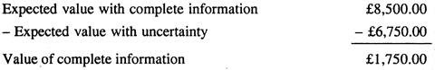
Thus, it is worth paying up to £1,750.00 to obtain as accurate an information as possible.

Choice under Uncertainty # 9. Demand for Risky Assets:

People are generally risk-averse. Given a choice, they prefer a fixed income to one that is as large on average that fluctuates randomly. Yet many of these people will invest all or part of their savings in stocks, bonds and other assets that carry some risk.

Why do risk-averse people invest in risky stocks either all or part of their investment? How do people decide how much risk to bear for the future? To answer these questions, we must examine the demand for risky assets.

Choice under Uncertainty # 10. Assets:

An asset is something that provides a monetary flow to its owner. The monetary flow from owning an asset can take the form of an explicit payment, such as the rental income from an apartment building. Another explicit payment is the dividend on shares.

But sometimes the monetary flow from ownership of an asset is implicit; it takes the form of an increase or decrease in the price or value of the asset — a capital gain or a capital loss.

A risky asset provides a monetary flow that is in part random, which means, the monetary flow is not known with certainty in advance. A share of a company is an obvious example of a risky asset — one cannot know whether the price of the stock will rise or fall over time, and one cannot even be sure that the company will continue to pay the same dividend per share.

Although people often associate risk with the stock market, most other assets are also risky.

The corporate bonds are example of this — the corporation that issued the bonds could go bankrupt and fail to pay bond owners their returns. Even long-term government bonds that mature in 10 or 20 years are risky.

Although it is unlikely that government will go bankrupt, the rate of inflation could increase and make future interest payments and the eventual repayment of principal worth less in real terms, and, thus, reduce the value of the bonds.

In contrast to risky assets, we can call an asset riskless if it pays a monetary flow that is certain. Short-term government bonds — known as Treasury Bills — are risk-free assets because they mature within a short period, there is very little risk of an unexpected increase in inflation.

And one can also be confident that government will not default on the bond. Other examples of riskless assets include passbook savings accounts in banks and building societies or short- term certificate of deposit.

Choice under Uncertainty # 11. Asset Returns:

People buy and hold assets because of the monetary flows they provide. Assets may be compared in terms of their monetary flow relative to the price of asset. The return on an asset is the total monetary flow it provides as a fraction of its value. For example, a bond worth £1,000 today that pays out £100 this year has a return of 10%.

When people invest their savings in stocks, bonds or other assets, they usually hope to earn a return that exceeds that rate of inflation, so that, by delaying consumption, they can consume more in the future. Thus, we often express the return on an asset in real terms which means return less the rate of inflation. For example, if the annual rate of inflation had been 5%, the bond would have yielded real return of 5%.

Since most assets are risky, an investor cannot know in advance what return they are going to yield in future. However, one can compare assets by looking at their expected returns which is just the expected value of its return. In a particular year, the actual return may be higher or lower than expected, but over a long period the average return should be close to the expected return.

Different assets have different expected returns. Table 5.6 shows that the expected real return on Treasury Bills has been less than 1%, while the real return for a representative stock on the London Stock Market has been almost 9%.

Why would a person buy a Treasury bill when the expected return on stocks is so much higher? The answer is that the demand for an asset depends not only on expected return, but also on its risk.

One measure of risk, the standard deviation (σ) of the real return, is equal to 21.2% for common stock, but only 8.3% for corporate bonds, and 3.4% for Treasury Bills, as Table 5.6 shows. Clearly, the higher the expected return on investment, the greater the risk involved. As a result, a risk-averse investor must balance expected return against risk.

Choice under Uncertainty # 12. Trade-Off between Risk and Return:

Suppose a person has to invest his savings in two assets — riskless Treasury Bills, and a risky representative group of stocks. He has to decide how much of his savings to invest in each of these two assets. This is analogous to the consumer’s problem of allocating a budget between two goods x and y.

Let us denote the risk-free return on the Treasury Bill by R_f, where the expected and actual returns are the same. Also, assume the expected return from investing in the stock market is R_m, and the actual return is Y_m.

The actual return is risky. At the time of investment decision, we know the likelihood of each possible outcome, but we do not know what particular outcome will occur. The risky asset will have a higher expected return than the risk-free asset (R_m > R_f) Otherwise, risk-averse investors would invest only in Treasury Bills and none at all in stocks.

To determine how much he will invest in each asset, let us assume b is the fraction of his savings placed in the stock market, and (1 – b) the fraction used to purchase Treasury Bills. The expected return on his total portfolio, R_p, is a weighted average of the expected return on the two assets

R_p = bR_m + (1 – b)R_f…………….. (2)

Suppose, the stock market’s expected return is 12%. Treasury Bills pay 4%, and b = 1/2. Then R_p = 8%. How risky is this portfolio? The riskiness can be measured by the variance of the portfolio’s return. Let us assume the variance of the risky stock market investment is σ²_m and the standard deviation is σ_m. We can show that the σ of the portfolio is the fraction of the portfolio invested in the risky asset times the o of that asset: σ_p = bσ_m……… (3)

Choice under Uncertainty # 13. Investor’s Choice Problem:

To determine how our investor should choose this fraction b, we must first show his risk- return trade-off analogous to the budget line of a consumer. To see this trade-off, we can rewrite equation (2) as

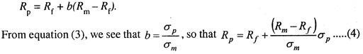
This is the budget line because it explains the trade-off between risk (σ_p) and the expected return (R_p). The slope R_m – R_f/σ_m is constant. The equation says that the expected return on the portfolio R_p increases as the standard deviation of that return σ_p increases.

The slope of the budget line is R_m – R/σ_m, which is the price of risk as shown in Fig. 5.3. Three indifference curves are drawn; each curve shows combinations of risk and return that have an investor equally satisfied. The curves are upward-sloping because a risk-averse investor will require a higher expected return if he is to bear a greater amount of risk. The utility-maximising investment portfolio is at the point where indifference curve U₂ is tangent to the budget line.

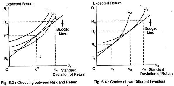
Choice under Uncertainty # 14. Two Different Investors Choice with Different Attitudes to Risk:

Investor A is risk-averse. His portfolio will consist mostly of the risk-free asset, so his expected return, R_A, will be only slightly greater than the risk-free return, but the risk σ_A will be small. Investor B is less risk-averse. He will invest a large fraction of his funds in stocks. The expected return on his portfolio, R_B, will be larger, but the return will also be riskier.