What is Aggregate Demand? | Employment | Economics

Get the answer of: What is Aggregate Demand?

National output or GNP as also the general price level are deter­mined by the interplay of aggregate demand and aggregate supply. This means that the total production of a country is determined partly by aggregate demand and partly by aggregate supply.

Aggregate demand refers to the quantity of goods and services that households, business firms and various government departments (at the central, state and local levels) are desirous of buying at existing prices. Likewise, aggregate supply refers to the quantity of goods and services that producing units (mainly business firms) want to offer for sale.

Aggregate demand (henceforth AD) refers to the total quantity of output that different economic units voluntarily buy at the existing price level, all other things remaining constant. In other words, AD is the desired expen­diture of society on existing goods and services.

It has the following four components:

1. Consumption:

Consumption (C) refers to expenditure on consumption goods personal consumption spending, largely depends on personal dis­posable income, i.e., personal income less taxes paid.

Various other factors also affect consumption spending such as perma­nent (or expected long term) income, household wealth, the general price level, as also the rate of interest. Aggregate consumption spending in macroeconomics refers to real consumption (i.e., nominal or rupee consump­tion divided by the price index for consumption goods).

2. Investment:

Private investment (J) refers to expenditure on capital goods such as plant, equipment and machinery. It also includes accumula­tion of inventories, i.e., stocks of finished goods, semi-finished goods (or goods-in-process) and raw materials.

The proximate determinants of invest­ment are expected rate of return on new investment, the rate of interest (which affects the cost of capital) as also rate of change of sales or of output of business firms. The central bank’s monetary (credit) policy also affects investment decisions by altering interest rates and credit availability.

3. Government expenditure:

The government’s current expenditure on goods and services (G) is the third important component of aggregate demand. Examples of this are Government purchase of food-grains from the farmers, Railway Board purchase of wagons, purchase of medicines by government hospitals, etc. The output of such goods, purchased by the government, adds to national income or GNP.

4. Net exports:

The fourth and final component of AD is net exports (X) which is the difference between the value of exports and the value of imports. Vari­ous factors affect imports such as domes­tic income and output, the ratio of domestic to foreign prices (called the terms of trade), and, of course, the for­eign exchange rate, i.e., rate of exchange of rupee in terms of another currency.

Since our imports are the exports of other countries, imports depend on the same set of factors such as foreign incomes and outputs, the terms of trade (or relative prices) and the foreign exchange rates. Since net exports are the difference between total exports and total imports, they depend on the same variables.

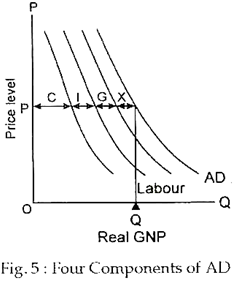
Fig. 5 shows a typical AD curve. The four components of AD are also shown separately. At the existing price level, P consumption is OC, invest­ment (CI), government expenditures (IC) and net export (GQ). All four components add up to Q. In other words, the four spending streams, at the existing price level together constitute AD.

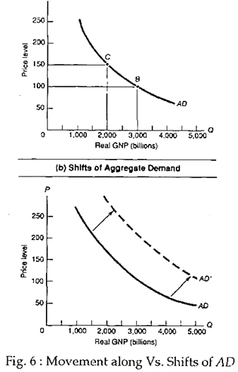
The AD curve in Fig. 5 shows the total real (or constant-price) expenditure at each price level, other things remaining the same. The AD curve, like all other demand curves, slopes downward from left to right. This means that aggregate real spending falls as the general price level rises. This point is illustrated in the upper part of Fig. 6.

This is usually explained by what is called the money-supply effect. This simply means that as the general price level rises, with total money supply remaining the same, the actual (real) de­mand for goods and services falls.

A fall in real money supply leads to a fall in consumption, investment and net export, i.e., to a decline in total spending. The end result is an upward move­ment along the AD curve from point A to B in the upper part of Fig. 6.

The AD curve may also shift to a new position, as shown in the lower part of Fig. 6. This may happen due to changes in gov­ernment’s monetary and fiscal policies or external factors such as fall in oil price, rise in share prices, or technological progress and output growth in foreign countries (which may lead to an increase in net exports).

In microeconomics a demand curve analyses the behaviour of an individual commodity. Such a demand curve is downward sloping due to price effect which is the sum total of income effect and substitution effect.

In contrast, the AD curve, used in macroeconomics, depicts changes in prices and output for the entire economy. Such a curve is downward sloping due to the money-supply effect.

Different economists hold different views regarding the determinants of aggregate demand. According to some economists, known as monetarists, the total stock of money in circulation is the primary determinant of the rupee value of spending.

One leading member of the monetarist school of thought, viz., Milton Friedman, holds the view that there is an exact propor­tional (fixed) relation between the rupee value of all purchases and the supply of money available. Thus, if total rupee spending is equated with nominal GNP, then nominal GNP will be proportional to the supply of money.

Another group of economists hold the view that the most important determinant of aggregate demand is income and spending flows. Thus, they focus on changes in government expenditure and tax programmes along with change in investment and economic conditions such as charges in the country’s balance of payments position as determinants AD and changes therein.

However, most modern economists like Samuelson, Lipsey, Baumol and others adhere to a new approach called an eclectic approach, holding that a wide variety of policy and external forces affect aggregate demand.

Aggregate Demand Curve:

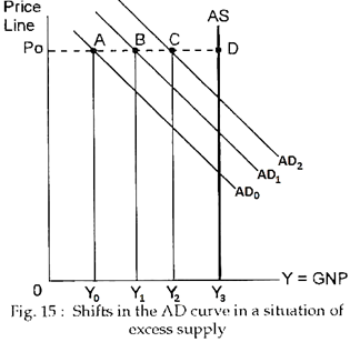
J.M. Keynes pointed out that when an economy has excess capac­ity, shifts in the aggregate demand curve result in different levels of output at the fixed price level, P₀. This point is illustrated in Fig. 15. Here POABCD is the aggregate supply curve and Y₃ is the potential (or full employment) output.

So long as the AS curve is completely elastic (a horizontal straight line) a rise in AD and rightward shift of the AD curve results in an increase in output from Y₀ to Y₁ to Y₂ and to Y₃. This is Keynes’ view of the Line macro-economy. And, the Keynesian model is a fix-price model.

In his theory of income deter­mination Keynes has shown how at any price level aggregate de­mand — and equilibrium output — is determined. By using the same analysis, it is possible to de­rive the aggregate demand curve simply by asking: what happens to aggregate demand — and equi­librium output — when the price level changes?

To answer this question, we have only to know how does the aggregate expendi­ture schedule shift when the price level rises or falls. When the price level rises, at each level of income, consumer will buy less goods and services, since their real income will fall.

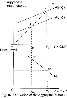
Moreover, if current price levels seem to be higher rela­tive to future price level (i.e., if prices are likely to fall in future), then households may reduce their current consumption (which has become relatively expensive). In this case, the aggregate expendi­ture schedule shifts downward and to the right, as shown in Fig. 16 and equilibrium output falls.

Thus, while Y₀ is output corre­sponding to the original price level P₀, as is indicated by the aggregate expenditure schedule AE (P₀), Y₁ is the new level of output corresponding to the new price level P₁. The top half of the diagram shows the effect of an increase in the price level from P₀ to P₁ on the aggregate expenditure schedule. It decreases equilibrium output from Y₀ to Y₁. The bottom half of the diagram traces out the equilibrium values of aggregate demand (and output) corresponding to different price levels.

Limitation:

The Keynesian theory has analysed the determination of national output by focusing exclusively as the aggregate expenditure sched­ule, which underlies the aggregate demand curve. However, aggregate supply is also important in a modern economy.

In Keynes’ model “changes in aggregate demand determine what happens to national output when there are idle machines and workers that could be put to work if only there were sufficient demand to purchase the goods they produced”.

However, as J. Stiglitz has rightly pointed out:

“There are many times when there is excess capacity in the country, and when the Keynesian approach, ignoring capacity constraints, makes perfect sense. There are other times, however, when the economy is working closer to capacity. Then only aggregate supply has to be brought into the picture.”