Iso-Quant Curve: Definitions, Assumptions and Properties

Iso-Quant Curve: Definitions, Assumptions and Properties!

The term Iso-quant or Iso-product is composed of two words, Iso = equal, quant = quantity or product = output.

Thus it means equal quantity or equal product. Different factors are needed to produce a good. These factors may be substituted for one another.

A given quantity of output may be produced with different combinations of factors. Iso-quant curves are also known as Equal-product or Iso-product or Production Indifference curves. Since it is an extension of Indifference curve analysis from the theory of consumption to the theory of production.

Thus, an Iso-product or Iso-quant curve is that curve which shows the different combinations of two factors yielding the same total product. Like, indifference curves, Iso- quant curves also slope downward from left to right. The slope of an Iso-quant curve expresses the marginal rate of technical substitution (MRTS).

Definitions:

“The Iso-product curves show the different combinations of two resources with which a firm can produce equal amount of product.” Bilas

“Iso-product curve shows the different input combinations that will produce a given output.” Samuelson

“An Iso-quant curve may be defined as a curve showing the possible combinations of two variable factors that can be used to produce the same total product.” Peterson

“An Iso-quant is a curve showing all possible combinations of inputs physically capable of producing a given level of output.” Ferguson

Assumptions:

The main assumptions of Iso-quant curves are as follows:

1. Two Factors of Production:

Only two factors are used to produce a commodity.

2. Divisible Factor:

Factors of production can be divided into small parts.

3. Constant Technique:

Technique of production is constant or is known before hand.

4. Possibility of Technical Substitution:

The substitution between the two factors is technically possible. That is, production function is of ‘variable proportion’ type rather than fixed proportion.

5. Efficient Combinations:

Under the given technique, factors of production can be used with maximum efficiency.

Iso-Product Schedule:

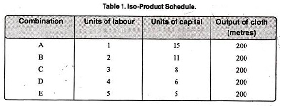
Let us suppose that there are two factor inputs—labour and capital. An Iso-product schedule shows the different combination of these two inputs that yield the same level of output as shown in table 1.

The table 1 shows that the five combinations of labour units and units of capital yield the same level of output, i.e., 200 metres of cloth. Thus, 200 metre cloth can be produced by combining.

(a) 1 units of labour and 15 units of capital

(b) 2 units of labour and 11 units of capital

(c) 3 units of labour and 8 units of capital

(d) 4 units of labour and 6 units of capital

(e) 5 units of labour and 5 units of capital

Iso-Product Curve:

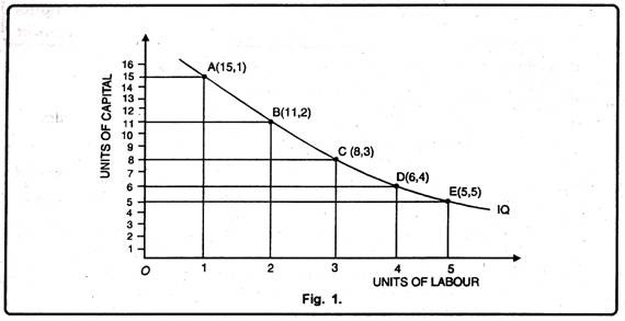
From the above schedule iso-product curve can be drawn with the help of a diagram. An. equal product curve represents all those combinations of two inputs which are capable of producing the same level of output. The Fig. 1 shows the various combinations of labour and capital which give the same amount of output. A, B, C, D and E.

Iso-Product Map or Equal Product Map:

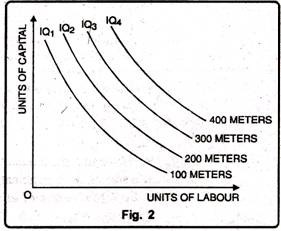
An Iso-product map shows a set of iso-product curves. They are just like contour lines which show the different levels of output. A higher iso-product curve represents a higher level of output. In Fig. 2 we have family iso-product curves, each representing a particular level of output.

The iso-product map looks like the indifference of consumer behaviour analysis. Each indifference curve represents particular level of satisfaction which cannot be quantified. A higher indifference curve represents a higher level of satisfaction but we cannot say by how much the satisfaction is more or less. Satisfaction or utility cannot be measured.

An iso-product curve, on the other hand, represents a particular level of output. The level of output being a physical magnitude is measurable. We can therefore know the distance between two equal product curves. While indifference curves are labeled as IC₁, IC₂, IC₃, etc., the iso-product curves are labelled by the units of output they represent -100 metres, 200 metres, 300 metres of cloth and so on.

Properties of Iso-Product Curves:

The properties of Iso-product curves are summarized below:

1. Iso-Product Curves Slope Downward from Left to Right:

They slope downward because MTRS of labour for capital diminishes. When we increase labour, we have to decrease capital to produce a given level of output.

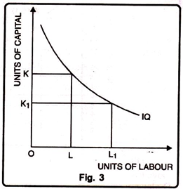
The downward sloping iso-product curve can be explained with the help of the following figure:

The Fig. 3 shows that when the amount of labour is increased from OL to OL₁, the amount of capital has to be decreased from OK to OK₁, The iso-product curve (IQ) is falling as shown in the figure.

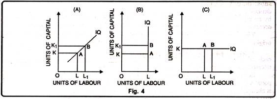
The possibilities of horizontal, vertical, upward sloping curves can be ruled out with the help of the following figure 4:

(i) The figure (A) shows that the amounts of both the factors of production are increased- labour from L to Li and capital from K to K₁. When the amounts of both factors increase, the output must increase. Hence the IQ curve cannot slope upward from left to right.

(ii) The figure (B) shows that the amount of labour is kept constant while the amount of capital is increased. The amount of capital is increased from K to K₁. Then the output must increase. So IQ curve cannot be a vertical straight line.

(iii) The figure (C) shows a horizontal curve. If it is horizontal the quantity of labour increases, although the quantity of capital remains constant. When the amount of capital is increased, the level of output must increase. Thus, an IQ curve cannot be a horizontal line.

2. Isoquants are Convex to the Origin:

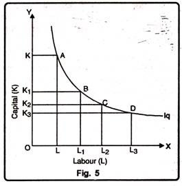
Like indifference curves, isoquants are convex to the origin. In order to understand this fact, we have to understand the concept of diminishing marginal rate of technical substitution (MRTS), because convexity of an isoquant implies that the MRTS diminishes along the isoquant. The marginal rate of technical substitution between L and K is defined as the quantity of K which can be given up in exchange for an additional unit of L. It can also be defined as the slope of an isoquant.

It can be expressed as:

MRTS_LK = – ∆K/∆L = dK/ dL

Where ∆K is the change in capital and AL is the change in labour.

Equation (1) states that for an increase in the use of labour, fewer units of capital will be used. In other words, a declining MRTS refers to the falling marginal product of labour in relation to capital. To put it differently, as more units of labour are used, and as certain units of capital are given up, the marginal productivity of labour in relation to capital will decline.

This fact can be explained in Fig. 5. As we move from point A to B, from B to C and from C to D along an isoquant, the marginal rate of technical substitution (MRTS) of capital for labour diminishes. Everytime labour units are increasing by an equal amount (AL) but the corresponding decrease in the units of capital (AK) decreases.

Thus it may be observed that due to falling MRTS, the isoquant is always convex to the origin.

3. Two Iso-Product Curves Never Cut Each Other:

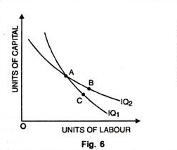
As two indifference curves cannot cut each other, two iso-product curves cannot cut each other. In Fig. 6, two Iso-product curves intersect each other. Both curves IQ1 and IQ2 represent two levels of output. But they intersect each other at point A. Then combination A = B and combination A= C. Therefore B must be equal to C. This is absurd. B and C lie on two different iso-product curves. Therefore two curves which represent two levels of output cannot intersect each other.

4. Higher Iso-Product Curves Represent Higher Level of Output:

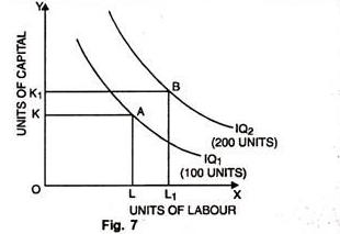
A higher iso-product curve represents a higher level of output as shown in the figure 7 given below:

In the Fig. 7, units of labour have been taken on OX axis while on OY, units of capital. IQ₁ represents an output level of 100 units whereas IQ2 represents 200 units of output.

5. Isoquants Need Not be Parallel to Each Other:

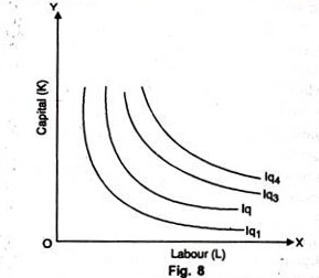
It so happens because the rate of substitution in different isoquant schedules need not be necessarily equal. Usually they are found different and, therefore, isoquants may not be parallel as shown in Fig. 8. We may note that the isoquants Iq₁ and Iq₂ are parallel but the isoquants Iq₃ and Iq4 are not parallel to each other.

6. No Isoquant can Touch Either Axis:

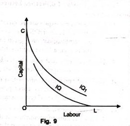
If an isoquant touches X-axis, it would mean that the product is being produced with the help of labour alone without using capital at all. These logical absurdities for OL units of labour alone are unable to produce anything. Similarly, OC units of capital alone cannot produce anything without the use of labour. Therefore as seen in figure 9, IQ and IQ₁ cannot be isoquants.

7. Each Isoquant is Oval-Shaped.

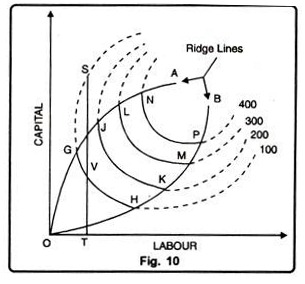
It means that at some point it begins to recede from each axis. This shape is a consequence of the fact that if a producer uses more of capital or more of labour or more of both than is necessary, the total product will eventually decline. The firm will produce only in those segments of the isoquants which are convex to the origin and lie between the ridge lines. This is the economic region of production. In Figure 10, oval shaped isoquants are shown.

Curves OA and OB are the ridge lines and in between them only feasible units of capital and labour can be employed to produce 100, 200, 300 and 400 units of the product. For example, OT units of labour and ST units of the capital can produce 100 units of the product, but the same output can be obtained by using the same quantity of labour T and less quantity of capital VT.

Thus only an unwise entrepreneur will produce in the dotted region of the iso-quant 100. The dotted segments of an isoquant are the waste- bearing segments. They form the uneconomic regions of production. In the up dotted portion, more capital and in the lower dotted portion more labour than necessary is employed. Hence GH, JK, LM, and NP segments of the elliptical curves are the isoquants.

Difference between Indifference Curve and Iso-Quant Curve:

The main points of difference between indifference curve and Iso-quant curve are explained below:

1. Iso-quant curve expresses the quantity of output. Each curve refers to given quantity of output while an indifference curve to the quantity of satisfaction. It simply tells that the combinations on a given indifference curve yield more satisfaction than the combination on a lower indifference curve of production.

2. Iso-quant curve represents the combinations of the factors whereas indifference curve represents the combinations of the goods.

3. Iso-quant curve gives information regarding the economic and uneconomic region of production. Indifference curve provides no information regarding the economic and uneconomic region of consumption.

4. Slope of an iso-quant curve is influenced by the technical possibility of substitution between factors of production. It depends on marginal rate of technical substitution (MRTS) whereas slope of an indifference curve depends on marginal rate of substitution (MRS) between two commodities consumed by the consumer.

Principle of Marginal Rate of Technical Substitution [June-2005]:

The principle of marginal rate of technical substitution (MRTS or MRS) is based on the production function where two factors can be substituted in variable proportions in such a way as to produce a constant level of output. The marginal rate of technical substitution between two factors C (capital) and L (labour), MRTS_LC is the rate at which L can be substituted for C in the production of good X without changing the quantity of output.

As we move along an isoquant downward to the right each point on it represents the substitution of labour for capital. MRTS is the loss of certain units of capital which will just be compensated for by additional units of labour at that point. In other words, the marginal rate of technical substitution of labour for capital is the slope or gradient of the isoquant at a point. Accordingly, slope = MRTS_LC = AC/AL. This can be understood with the aid of the isoquant schedule, in Table 2.

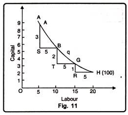
The above table 2 shows that in the second combination to keep output constant at 100 units, the reduction of 3 units of capital requires the addition of 5 units of labour, MRTS_LC = 3 : 5. In the third combination, the loss of 2 units of capital is compensated for by 5 more units of labour, and so on.

In Fig. 11 at point B, the marginal rate of technical substitution is AS/SB, t point G, it is BT/TG and at H, it is GR/RH. The isoquant AH reveals that as the units of labour are successively increased into the factor- combination to produce 100 units of good X, the reduction in the units of capital becomes smaller and smaller.

It means that the marginal rate of technical substitution is diminishing. This concept of the diminishing marginal rate of technical substitution (DMRTS) is parallel to the principle of diminishing marginal rate of substitution in the indifference curve technique. This tendency of diminishing marginal substitutability of factors is apparent from Table 2 and Figure 11.

The MRTS_Lc continues to decline from 3: 5 to 1: 5 whereas in the Figure 11 the vertical lines below the triangles on the isoquant become smaller and smaller as we move downward so that GR < BT < AS. Thus, the marginal rate of technical substitution diminishes as labour is substituted for capital. It means that the isoquant must be convex to the origin at every point.

Iso-Cost Line:

The iso-cost line is similar to the price or budget line of the indifference curve analysis. It is the line which shows the various combinations of factors that will result in the same level of total cost. It refers to those different combinations of two factors that a firm can obtain at the same cost. Just as there are various isoquant curves, so there are various iso-cost lines, corresponding to different levels of total output.

Definition:

Iso-cost line may be defined as the line which shows different possible combinations of two factors that the producer can afford to buy given his total expenditure to be incurred on these factors and price of the factors.

Explanation:

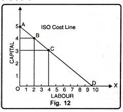
The concept of iso-cost line can be explained with the help of the following table 3 and Fig. 12. Suppose the producer’s budget for the purchase of labour and capital is fixed at Rs. 100. Further suppose that a unit of labour cost the producer Rs. 10 while a unit of capital Rs. 20.

From the table cited above, the producer can adopt the following options:

(i) Spending all the money on the purchase of labour, he can hire 10 units of labour (100/10 = 10)

(ii) Spending all the money on the capital he may buy 5 units of capital.

(iii) Spending the money on both labour and capital, he can choose between various possible combinations of labour and capital such as (4, 3) (2, 4) etc.

Diagram Representation:

In Fig. 12, labour is given on OX-axis and capital on OY-axis. The points A, B, C and D convey the different combinations of two factors, capital and labour which can be purchased by spending Rs. 100. Point A indicates 5 units of capital and no unit of labour, while point D represents 10 units of labour and no unit of capital. Point B indicates 4 units of capital and 2 units of labour. Likewise, point C represents 4 units of labour and 3 units of capital.

Iso-Cost Curves:

After knowing the nature of isoquants which represent the output possibilities of a firm from a given combination of two inputs. We further extend it to the prices of the inputs as represented on the isoquant map by the iso-cost curves.

These curves are also known as outlay lines, price lines, input-price lines, factor-cost lines, constant-outlay lines, etc. Each iso-cost curve represents the different combinations of two inputs that a firm can buy for a given sum of money at the given price of each input.

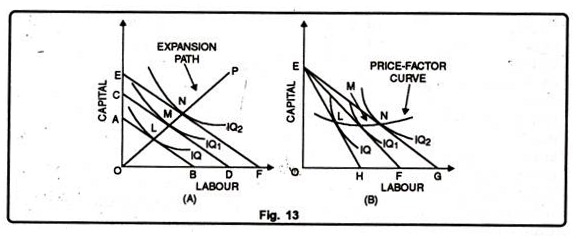
Figure 13 (A) shows three iso-cost curves each represents a total outlay of 50, 75 and 100 respectively. The firm can hire OC of capital or OD of labour with Rs. 75. OC is 2/3 of OD which means that the price of a unit of labour is 1/2 times less than that of a unit of capital.

The line CD represents the price ratio of capital and labour. Prices of factors remaining the same, if the total outlay is raised, the iso-cost curve will shift upward to the right as EF parallel to CD, and if the total outlay is reduced it will shift downwards to the left as AB.

The iso-costs are straight lines because factor prices remain the same whatever the outlay of the firm on the two factors.

The iso-cost curves represent the locus of all combinations of the two input factors which result in the same total cost. If the unit cost of labour (L) is w and the unit cost of capital (C) is r, then the total cost: TC = wL + rC. The slope of the iso-cost line is the ratio of prices of labour and capital i.e., w/r.

The point where the iso-cost line is tangent to an isoquant shows the least cost combination of the two factors for producing a given output. If all points of tangency like LMN are joined by a line, it is known as an output-factor curve or least-outlay curve or the expansion path of a firm.

It shows how the proportions of the two factors used might be changed as the firm expands. For example, in Figure 13 (A) the proportions of capital and labour used to produce 200 (IQ₁) units of the product are different from the proportions of these factors used to produce 300 (IQ₂) units or 100 units at the lowest cost.

Like the price-income line in the indifference curve analysis, a relative cheapening of one of the factors to that of another will extend the iso-cost line to the right. If one of the factors becomes relatively dearer, the iso-cost line will contract inward to the left.

Given the price of capital, if the price of labour falls, the isocost line EF in Panel (B) of figure 13 will extend to the right as EG and if the price of labour rises, the iso-cost line EF will contract inward to the left as EH, if the equilibrium points L, M, and N are joined by a line. It will be called the price-factor curve.

Ridge Lines:

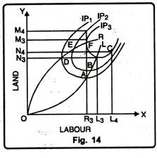
One knows from the iso-quant curves the extent to which production should be carried out. Lines which represent the limits of the economic region of production are called ridge lines. Ridge lines join those points on different iso-quant curves which determine the economic limits of production. The importance of ridge lines is explained with the help of Figure 14.

Iso-quant curves at point A and D; B and E; and C and F begin to recede from each axes. The segments above or below these points A B C and D E F, one gets OL and OR lines. OR and OL lines are called Ridge Lines. These ridge lines show the economical limits for the firm to produce only in those segments of the iso-quants which lie between the ridge lines.

It can be explained with the help of an example. In fig. 14, combination of OL3 units of labour and ON3 units of land can produce 60 quintals of wheat, ON3 amount of land is the minimum required to produce 60 quintals of wheat.

While using ON₃ amount of land, at point C, if more than OL₃ units of labour are used, total output will be less than 60 quintals of wheat. It means beyond OL3 units of labour, their marginal productivity will become negative causing total output to be less than 60 quintals. In other words, after OL₃, marginal productivity of labour will be zero.

If at point ‘C’ more than OL₃ units of labour are used then to keep the total output of 60 quintals of wheat constant, more than ON3 units of land will have to be used. It will be unwise and irrational decision. It will unnecessarily increase the cost of production. Thus to produce outside point ‘C’ will be uneconomic. At point ‘C’ marginal productivity of labour will be zero.

In the same way, we can find out point A and B on iso-quant curves IP) and IP2 where marginal productivity of labour will be zero. The lines joining these points are called ridge lines. Ridge line OL, therefore, is the locus of points where marginal productivity of labour is zero. Point F of IP3 indicates that to produce 60 quintals of wheat, OR3 units of labour and OM3 units of land are required. OR3 units of labour are the minimum units to produce this level of output. If keeping OR3 units of labour constant, more than OM3 units of labour are used, the total output will be less than 60 quintals of wheat. It implies that after point ‘F’.

Accordingly, points ‘D’ and ‘E’ on IPi and IP2 curves represent zero marginal productivity of land. Production thus, will be done on the segment below point ‘D’, ‘E’ and ‘F’. These points have been joined by OR ridge line.

Producer’s Equilibrium or Optimum Combi­nation of Factors or Least Cost Combination:

In simple words, producer’s equilibrium implies to that situation in which producer maximizes his profit. In short, the producer is producing given amount of output with least cost combination of factors. It is also known as optimum combination of the factors.

Optimum combination is that combination at which either:

(i) The output derived from a given level of inputs is maximum or

(ii) The cost of producing given output is minimum.

For producer’s equilibrium or optimum combination, it must fulfill following two conditions as:

(i) At the point of equilibrium the iso-cost line must be tangent to isoquant curve.

(ii) At point of tangency i.e., iso-quant curve must be convex to the origin or MRTS_Lk must be falling.

The iso-cost line gives information regarding factor prices and financial resources of the firm.

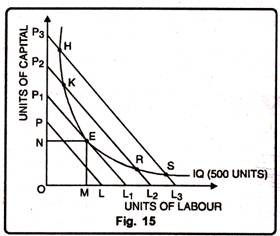
With a given outlay and prices of two factors, the firm obtains least cost combination of factors, when the iso-cost line becomes tangent to an iso-product curve. Let us explain it with the following Fig. 15.

In Figure 15, P₁L₁ iso-cost line has become tangent to iso-product curve (representing 500 units of output) at point E. At this point, the slope of the iso-cost line is equal to the iso-product curve. The slope of the iso- product curve represents MRTS of labour for capital. The slope of the iso-cost line represents the price ratio of the two factors.

Slope of Iso-quant curve = Slope of Iso-cost curve

MRTS_Lk = – ∆L/∆L = MP_L/MP_K = P_L/P_K

[where ∆K → change in capital, ∆L → change in labour, MPL → Marginal Physical Product of Labour, MPk – Marginal Physical Product of capital, P_L Price of Labour, and P_K → Price of capital, MRTS_LK ⁼ Marginal Rate of Technical Substitution of labour and capital.]

The firm employs OM units of labour and ON units of capital. The producing firm is in equilibrium. It obtains least cost combination of the two factors to produce 5 00 units of the commodity.

The points such as H, K, R and S lie on higher iso-cost lines. They require a larger outlay, which is beyond the financial resources of the firm.

The same can be explained with the help of a numerical example. Suppose the firm decides to produce 10 units of output. The two factors are labour and capital. The price of labour per hour is Rs. 10 and the price of machine use per hour is Rs. 10. The following table shows the various combinations of labour and machine capital hours required to produce 10 units of output.

It is clear from this table that the least cost of production is P2. A rational producer will chose this combination of factors, given the factor prices. Expansion path means locus of all such points that shows least cost combination of factors corresponding to different levels of output.

Expansion Path:

As financial resources of a firm increase, it would like to increase its output. The output can only be increased if there is no increase in the cost of the factors. In other words, the level of total output of a firm increases with increase in its financial resources.

By using different combinations of factors a firm can produce different levels of output. Which of the optimum combinations of factors will be used by the firm is known as Expansion Path. It is also called Scale-line.

“Expansion path is that line which reflects least cost method of producing different levels of output.” Stonier and Hague

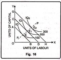
Expansion path can be explained with the help of Fig. 16. On OX-axis units of labour and on OY-axis units of capital are given.

The initial iso-cost line of the firm is AB. It is tangent to IQ at point E which is the initial equilibrium of the firm. Supposing the cost per unit of labour and capital remains unchanged and the financial resources of the firm increase.

As a result, firm’s new iso-cost-line shifts to the right as CD. New iso-cost line CD will be parallel to the initial iso-cost line. CD touches IQ₁ at point E₁ which will constitute the new equilibrium point. If the financial resources of the firm further increase, but cost of factors remaining the same, the new iso-cost line will be GH.

It will be tangent to Iso-quant curve IQ2 at point E₂ which will be the new equilibrium point of the firm. By joining together equilibrium points E, E₁ and E₂, one gets a line called scale-line or Expansion Path. It is because a firm expands its output or scale of production in conformity with this line.

Isoquant Curve and Returns to a Factor:

Returns to a factor refers to the behavior of output in response to changing application of one factor of production while other factors remaining constant. As in the case of returns to scale, there are three different aspects of returns to a factor, viz., increasing returns, constant returns and diminishing returns.

The returns to a factor can be explained using isoquant techniques. It is assumed that capital is a fixed input and labour is a variable input.

Different Stages of Returns to a Factor:

The different returns to a factor can be explained as follows:

(i) Increasing Returns to a Factor:

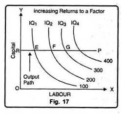
It occurs when additional application of the variable factor i.e., labour increases total output at increasing rate. Fig. 17 explains the situation of increasing returns to a factor.

In Fig. 17 capital is taken constant at OR units. The line RP shows how larger quantities of labour can be employed to expand production. It is called output path.

The isoquant curves for 100, 200, 300 and 400 units of output shows that output is increasing by a constant amount by 100 units. These isoquants intersect the output path RP at point E, F, G and H.

We see here that the distance between successive isoquant curves is decreasing, that is, less and less labour is needed for every additional 100 units of output. This means an increasing marginal product of labour. However, the distance EF is greater than FG and FG is greater than GH i.e.

EF = FH = GH

This means that 100 units increase in output can be obtained by employing successively lesser increments of labour. Let us suppose that EF is 20 units of labour and FG is 10 units of labour. Then from E to F the additional 100 units of output are obtained by employing additional 20 units of labour. From F to G additional 100 units of output is obtained by employing only 10 more units of labour. In short, the marginal product of labour increases when output is expanded along the output path RP.

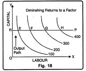
(ii) Diminishing Returns to a Factor. Diminishing returns to a factor is a situation when increasing application of the variable factor increases total output only at the diminishing rate.

Fig. 18 illustrates the situation of diminishing rate. When capital is taken constant at OR and production is expanded by adding more labour, the distance between successive Isoquants becomes increasingly greater, that is even more and more labour is needed for every additional 100 units of output. This shows a diminishing marginal product of labour. The distance EF is less than FG and FG is less than GH.

EF < FG < GH Thus, 100 units increase in output can be obtained only by employing successively greater increments of labour. Between E to F additional 100 units of output is obtained by applying additional 10 units of labour. Between F to G additional 100 units of output is obtained by applying additional 20 units of labour. Therefore, the marginal product of labour diminishes when output is expanded along the output path RP.

(iii) Constant Returns to a Factor:

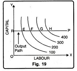
A constant return to a factor occurs when increasing application of the variable factor increases total output only at a constant rate. Fig. 19, we see that when capital is taken constant at OR and production is increased by adding more labour, the distance between isoquants remains constant, so that same amount of labour is needed for every additional 100 units of output.

This means a constant marginal product (MP) of labour. In other words, 100 units increase in output can be obtained by employing equal increment of labour. The distance between different iso-quants remains equal. It can be written as;

EF = FG = GH

Difference between Returns to Scale and Returns to a Factor:

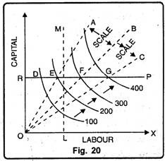
With the help of Isoquant diagram, we can draw the difference between returns to scale and returns to factor. Returns to scale implies that output is increased as all the inputs are increased in the same proportion. However, Fig. 20 shows difference between returns to scale and returns a factor.

In Fig. 20 on OX-axis labour is measured and on OY-axis capital. We draw straight lines OA, OB and OC through the origin. These lines or rays show that both labour and capital are increased to expand output. Moreover, since the lines OA, OB and OC are straight lines passing through the origin, the ratio between labour and capital remains same along each one of these lines.

Moving along a ray like OA means to increase production or scale always with the same ratio of inputs. For instance the isoquants in Fig. 20 show constant returns to scale. The isoquants for 100, 200, 300 and 400 units of output intersect the straight lines OA, OB and OC at equal distance.

Thus; it requires twice as much of both capital and labour to produce 200 units instead of 100 units; 50 percent further more to produce 300 instead of 200 and so on. In other words the rays show the returns to scale which implies that to increase output both the inputs should be increased in the same proportion.

Returns to a factor or change in proportion refers one input is held constant while production is expanded by increasing the quantity of the other input. The horizontal straight line RP is drawn on the assumption that capital is kept constant at OR and production expanded by adding more labour. The vertical straight line LM is drawn on the assumption that labour is held constant at OL and output is expanded by adding more capital.

As we move along these lines the amount of one input varies while of the other remains constant. Thus proportion between the two outputs undergoes a change. The returns to a factor can be explained either by RP line or LM line depending whether capital is held constant or labour is held constant. With capital constant at R; the producer moves from to E, from E to F to G.

Therefore, the successive difference between the isoquants is increasing (FG > EF). This means that 100 units of additional output can be obtained by employing successively greater increments of labour. This means diminishing marginal product of labour. This is the case of diminishing returns to a factor. In short, both the concepts of returns to scale and returns to a factor (change in factor proportions) can be explained by using the technique of Isoquants.