
The following points highlight the top three techniques of economic forecasting in business. The techniques are: 1. Methodology 2. Industry Forecasting 3. Firm’s Product Demand Forecasting.
Technique # 1. Methodology:
Various economic forecasting techniques are available. They range from simple and relatively inexpensive procedures to methods that are quite complex, highly sophisticated and very expensive. Some of the techniques are quantitative while others are qualitative. It is very difficult to say which one is the best. The best one for a particular task depends on the specific nature of the forecasting problem.
Some of the relevant factors that are to be considered here include the following:
1. The time into the future that one must forecast.
ADVERTISEMENTS:
2. The degree of accuracy required.
3. The lead time available before arriving at a decision.
4. The quality of data available for the purpose of analysis.
5. The nature of relationships included in the forecasting problem.
ADVERTISEMENTS:
6. The benefits expected from a successful forecast compared to the costs associated with using a particular technique.
Some techniques are quite satisfactory for short run projections, such as barometric and survey methodology. Others require more lead time and are thus more useful for long-run forecasting. Moreover, within each class of forecasting technique, the level of sophistication varies enormously.
It is anybody’s guess that the more sophisticated techniques are also more expensive. Therefore, in choosing among techniques of varying degrees of sophistication, the forecaster should consider the trade-off between (the benefits of) greater accuracy” and the additional cost (of achieving this accuracy).
For example, if the forecaster “expects that an accurate forecast would leave him with a large stock of unsold goods, he should consider reducing the risk of suffering potential losses by paying for greater accuracy. If greater accuracy saves him only small amounts in losses, he may find that greater accuracy is not worth the extra expense.”
ADVERTISEMENTS:
We may now discuss some of the forecasting methods currently in use. The forecaster must assess the strengths and weaknesses of each technique in order to choose the best technique for his particular problem.
All these techniques are useful for forecasting demand for well-established (old) products. New products create complications because no reliable data are available for the purpose. We shall first discuss the technique of forecasting the demand for old products.
i. Survey of Buyers’ Intentions:
The method is used for short-term forecasting. The method seeks to “determine whether potential customers intend to buy a certain product or service in the forecasting period. An attempt may be made with this method also to ascertain how many units of a product a customer will buy and at what prices.”
Some forecasters also make a survey of consumer intentions. Intention surveys are used to judge the level of confidence the consumer feels concerning the desirability of spending for consumption in the future.
If consumers are hesitant about continuing their purchases of consumer durables like T.V. sets or semi-durables like clothing in the new or medium future due to pessimistic expectations about the state of the economy (and indirectly the likelihood of their incomes remaining at high levels), we might forecast a fall in the demand for these products in future periods.
For non-durables such as food, the consumers’ purchases may be expected to continue at a relatively constant level almost regardless of the level of aggregate economic activity.
However, for durables and semi-durables, the consumer may postpone such purchases if the immediate outlook is less promising. If consumer expectations suddenly become pessimistic, we would expect the demand for such products to fall in the near future.
Some firms selling capital goods, or whose main customers are other firms, also make a summary of investors’ intentions. Such intentions have important implications for the demand for a variety of products such as construction materials, office supplies, and plant and equipment.
Investors’ intentions are highly dependent upon their expectations as to the future level of aggregate activity. Investors will feel more confident about investing if they expect aggregate activity to remain high or increase from its present level, since this has implications for the degree of idle capacity in future periods.
ADVERTISEMENTS:
If, on the contrary, the investors’ expectations are relatively pessimistic, we might expect investment projects to be postponed or cancelled, with subsequent impacts upon the level of aggregate economic activity.
A continuing survey of intentions does serve, however, as an on-going ‘finger on the pulse’ of the people who make the demand decisions. Any change in the expectations of these decision makers, and by association, a change in expected future demand levels, should become immediately apparent.
Thus decision makers have an advance warning of likely changes and can plan their production, inventories and other matters more effectively.
As a general rule, surveys are “based on interviews or questionnaires that ask individuals to reveal their future plans. Since businesses normally plan and budget their purchases in advance, surveys may reveal the impact of these decisions on one’s own company. While most consumers make many last-minute buying decisions, they often plan for major purchases of houses, automobiles, education and trips in advance.”
ADVERTISEMENTS:
For sporadic or perennial sales items, such as automobiles, suits, and foodstuffs a survey may be taken of the past purchases. In case of houses, a survey may be made among potential buyers.
Strengths & Weaknesses:
Survey methods are widely used because they provide useful supplementary material in addition to more highly quantitative techniques. In fact, econometric methods, which are used for quantitative forecasts, depend on an underlying stability of the relation between the major demand determinants and the quantity demanded.
These quantitative techniques often fail to capture the more emotionally and psychologically based swings in consumer behaviour. But a carefully constructed survey method may clearly reveal this type of information.
ADVERTISEMENTS:
D. Salvatore has made an overall assessment of this technique in the context of U.S.A. in these words: “In general, the record of these surveys has been rather good in forecasting actual expenditures, except in a few years of unexpected international political upheavals such as war or the threat of war. When used in conjunction with other quantitative methods, surveys can thus be very useful in forecasting economic activity in specific sectors of the economy and for the economy as a whole.”
However, this method is not free from defects. The longer the forecast period, the greater the chances of error. So this method is unlikely to give accurate results.
ii. Forecasting Turning Points — Barometric Forecasting:
Economic forecasters, especially in the U.S.A., have always tried to search out or identify certain indicators of a change in economic activity. A general business indicator “is a series of indexes of several different business activities combined into one general index of business activity”.
There is, of course, no simple indicator which even provides a consistent signal for change. But there are well known time series that have served as barometers of change. Barometric forecasting is “the prediction of turning points in one economic time series through the use of observations on other time series called barometers or indicators.”
The pioneering work in this area has been done by the economists at the National Bureau of Economic; Research (USA). They have classified economic time series into three broad categories: leading indicators, coincident indicators and lagging indicators. These indicators provide signals or indications of changes in economic activity, such as national income, or national product, the level of employment or the rate of price inflation.
These statistical indicators include 25-indexes, each measuring a different aspect of economic activity, selected originally by U.S.A.’s National Bureau because of their strong correlation with the general level of business activity.
ADVERTISEMENTS:
The group of leading indicators including 12 indexes whose turning points, upward and downward, usually precede peaks (upper turning points) and troughs (lower turning points) in the general level of business activity. The group of coincident indicators consist of 6 other indexes whose turning points usually correspond with the peaks and troughs in the general level of business activity.
Finally, there are 7 lagging indicators, where turning points do occur after the turning points in the general level of business activity. These 25 indicators together with their mean lead (-) and lag (+) time (in months) with respect of the actual cyclical peak or trough, are listed in table 1.


Source:
U.S. Department of Commerce, Bureau of Economic Analysis, Handbook of Cyclical Indicators (Washington, D.C.: Government Printing Office, May 1977), pp. 174-191. These economic indicators are published in the USA on a weekly basis. When plotted in a diagram the relative position of these indicators look like the one in Fig. 1.

Fig. 1 shows that leaders lead and lagers lag. We also see that “leading indicators precede (lead) business cycles turning points (i.e., peaks and troughs), coincident indicators move in step with business cycles, while lagging indicators follow or lag turning points in business cycles.”
Leading indicators do not always give a clear- cut indication of turn in economic activity. As S. H. Hymans has observed, “the index of leading indicators used by the U.S. government predicted all ten turning points between 1948 and 1970, but also predicted 24 peaks that did not occur. Moreover, these indexes are not quite accurate in predicting the exact timing of the turning points.”
This method is expensive also. However, in spite of these conceptual and practical difficulties, these methods are being widely used and promising search is being done in this area.
iii. Index Numbers- Composite and Diffusion Indexes:
Composite and diffusion indexes often overcome, at least partly, the difficulties in barometric forecasting and are also used for forecasting purpose.
Composite indexes (indicators) are those that measure several aspects of business activity by covering a wide range of economic activities. They are thus quite reliable business cycle indicators. Table 1, therefore, gives the lead and lag time for the Composite indexes of 12 leading, the 4 roughly coincident, and the 6 lagging indicators.
The most outstanding of the indexes are: industrial production, gross national product, and capacity utilization rate. They are weighted averages of several leading indicators in each group. Large weights are given to those indicators which do the job of forecasting better than others.
ADVERTISEMENTS:
As such, such indexes offer an important advantage: they smooth out random fluctuations, or noise, and provide more reliable forecasts and fewer wrong signals of changes in the predicted variable, than individual indicators.
In order to overcome the difficulty arising when some of the 12 leading indictors move up and some move down, another method is used. This is known as the diffusion (pressure) index. Rather than combining 12 leading indicators into a composite index, economists construct a diffusion index (DI) which gives the percentage of the 12 leading indicators moving upward.
As Pappas has put it, “instead of combining a number of leading indicators into a single standardized index, the methodology consists of noting the percentage of the total number of leading indicators that are rising ‘at a given point of time.” If, for instance, as the 12 leading indicators move up at the same time, DI is 100.
If, at the other extreme, they all go down, DI is zero. If only 6 move up, the DI would be (6/12) (100), or 50. A diffusion index, indicates the percentage of those leading indicators that is increasing at the present time. Usually an economist forecasts an improvement in economic activity when the value of DI exceeds 50. If it is closer to 100, the forecaster will have greater confidence in his forecast.
As a general rule, barometric forecasting is largely based on composite and diffusion indexes. Not much reliance is placed on individual indicators, except when a firm needs information about expected changes in the market for certain specific goods and services.
The U.S. Department of Commerce reports change in the individual and composite indexes every month. It may apparently seem that individual monthly swings are not very significant for studying business cycles.
ADVERTISEMENTS:
Yet, as Salvatore has opined, “three or four successive one-month declines in the composite index and a diffusion index of less than 50% are usually a prelude to recession or a slowing down of economic activity.”
This point is illustrated in Fig. 2. The top half of the diagram indicates that the composite index of leading indicators turned down prior to (i.e., lead) the recessions of 1969 to 1970, 1973 to 1975, and 1981 and 1982.
The shaded areas in the figure show those recessions. The bottom half makes it clear that the diffusion index for the 12 leading indicators was generally below 50% in the months preceding the recessions (the shaded areas).

Shortcomings:
The composite and diffusion indexes (of leading indicators) are no doubt acceptable tools for macro-level forecasting, i.e., for predicting turning points in business cycles. But there are certain shortcomings of this method. Firstly, on various occasions economists forecasted a recession that failed to occur. Secondly, there can be considerable variability in lead time.
Thirdly, and more importantly, this index number method (of barometric forecasting) “gives little or no indication of the magnitude of the forecasted change in the level of economic activity (i.e., it provides only a qualitative forecast of turning points)”.
Thus, although it is superior to the time series analysis and other smoothing techniques in forecasting short-run turning points in economic activity, it has to be used in conjunction with econometric methods in order to forecast the quantum of change in the level of business activity.
iv. Econometric Models:
The statistical methods used in forecasting can be broadly sub-divided into two categories, namely, time series models and econometric models. The primary distinguishing characteristics of econometric models is the use of an explicit structural model that attempts to explain the underlying economic relations.
To be more specific if we wish to employ an econometric model to forecast future sales it is necessary to develop a model that incorporate those variables that actually determine the level o sales (e.g. income, the price of substitutes and so on.)
In this type of quantitative approach some loose relation is established between sales and some leading indicators, whereas in the time series approach, sales are assumed to behave in some regular fashion over time.
In reality different economic variables are found to be interrelated. Therefore, a single equation is grossly inadequate to represent the factors that determine sales. So there is need to develop a multiple equation model that incorporates a system of equations to explain the interaction that underlies the demand level at any particular point of time.
By plugging in the forecast values for independent variables and assuming that the co-efficient discovered in an earlier testing will be a reliable indicators of future relationship, it is possible to solve the system of simultaneous equations to forecast the level of demand in future time periods.
Suppose that we have found the level of sales to be estimated fairly accurately by the system of equations:
St = -aPt + bYt ……. (1)
Pt/Yt = cYt-1 .…….(2)
Yt = Y0(1 + k)t ……..(3)
In this simple model current sales are a function of current prices and income levels (equation 1) but current prices and income are, in their turn, functions of past income levels (equation 2).
Since income is assumed to grow at constant rate k(equation 3), it is possible to project future income levels and future price levels. Thus on the basis of the estimate of parameters a, b, c, and k it is possible to project the level of sales in future periods.
Econometric models have three major advantages for forecasting purposes. Firstly, econometrics require analysts to define explicit causal relations. This specification by an explicit model enables the forecaster to search out or identify correlations between normally unrelated variables and may help to make the model more logically consistent and reliable.
Secondly, such models permit analysts to consider the sensitivity of the variable to be forecasted, to the changes in the exogenous variables. Using estimated values it is possible to determine which of the variables are most important in determining changes in the variables to be forecasted. Therefore, the analyst will know how to watch the behaviour of these variables more closely.
Thirdly, this approach can easily be used for computer simulation. A simulation model basically permits researchers to consider alternative projection based on hypothetical conditions. Thus analysts could get a clear idea of what could happen if market conditions changed.
v. Input-Output Forecasting:
Input-output forecasts are generated by using a device known as the input-output table developed by W. Leontief. Basically an input-output table is a matrix, each area of which shows an output or sales of a particular sector of the economy. In the same way each column indicates all the input used by a particular sector of the economy. All figures are in terms of money.
Input-output analysis is an attempt to reveal the structural interdependence of the economic system. Input-output analysis for an entire economy is based on an accounting of the flow of goods and services in rupee terms at a particular time.
Part of this flow is an inter-industry flow, goods transferred from an industry to be used in the production, processes of other industries, and the remainder flows to an exogenously defined, ‘final demand’ sector.
This sector generally includes households, government, and foreign trade, often lumped together. To be precise, an input-output table shows the purchases by a particular sector from all the other sectors, and sales by the sector to the other sectors.
The table below shows a very simple hypothetical input-output table:

If we consider the output of industry X worth Rs. 200, we notice that Rs. 60 worth of X was purchased by industry Y, Rs. 40 worth by industry Z and Rs. 100 worth by final consumers. In a like manner, to produce the output, industry X purchased Rs. 40 worth of output from industry Y, Rs. 50 worth from industry Z, and Rs. 110 of labour services.
From the above table we can construct another table which shows the corresponding input coefficients:

The table above shows the amount of output that needs to be purchased from the various sectors to produce one unit of output for a particular sector. Thus the first column shows that to obtain Re. 1 worth of output from industry X requires purchase of Re. 0.2 worth of output from Y, Re. 0.25 worth from Z and Re. 0.55 of labour services.
If some simplifying assumptions are made, the uses of this type of analysis are considerable. For example, one may like to know what the effect would be of an increase in final demand for the product of industry X to Rs. 120, other final demands remaining constant. Thus we make an assumption regarding consumer demand.
Prices are also assumed to remain unchanged as also the input coefficients. The last assumption follows from the postulate of constant returns to scale. So factor substitution either due to changes in the relative prices of inputs or changes in technology is ruled out.
The answers to our query can be found by solving the three simultaneous equations given below where x, y and z are the output in Rs. from industry X, Y and Z. It is obvious that all three outputs will change due to structural interdependence.
x = 0.15y + 0.2z + 120 ……… (1)
y = 0.2x + 05z + 260 …….. (2)
z = 0.25x + 0.25y + 50 ……… (3)
Equation (18.4), for example, tells us the demand that are made upon the output of industry X by industry Y, Z and final consumers. The solution of the equations are :
x = Rs. 222, y = Rs. 408 and z = Rs. 208.
These show the amount of new output required to satisfy intermediate and final demands. A final step would be to work out the new demand for labour services to see if this is feasible in view of known resources.
Input-output analysis is a variable tool to the forecaster because it gives a total picture of the markets for any group of commodities.
Moreover, forecasts that are generated by this technique are internally consistent, making it possible for the forecaster to determine what effect changes in demand will have on different industries. Finally, as input-output tables give a total picture of various market commodities, it also often indicates possible independent variables that may be used in regression analysis.
Uses and Shortcomings of Input-Output Forecasting:
Input-output models have various uses and abuses. Prima facie, such models are used by companies to forecast the raw materials, labour power and capital requirements needed to meet a forecasted change in the demand for their products.
However, input-output models are based on two unrealistic assumptions.
First input coefficients are assumed to remain fixed and so the possibility of factor-substitution is ruled out.
Secondly, the assumption of constant prices of commodities rules out the possibility of substitution in consumption. In spite of such defects, “there is stress on input output analysis and forecasting, because they take into consideration the interrelationships among the various industries and sectors of the economy in an internally consistent manner.”
vi. Judgmental Forecasting of Macroeconomic Activity:
Some forecasters rely largely, if not entirely, on judgement to derive future values of aggregate economic quantities. Although forecasting is both an art and science, judgemental forecasts represent the last step in the art of forecasting. By using his own knowledge and experience, the forecaster is able to analyse various key sectors in the economy. Forecasts are generated for the key sectors on the basis of such analysis.
In general, the sectors that are evaluated represent the components of GNP so that a forecast of the aggregate of this aggregate economic quantity is obtained by combining the forecasts of the component sectors.
Short comings:
Judgemental forecasts have limited value because it is extremely difficult for even the most experienced and knowledgeable economist to generate forecasts by sectors, that are consistent.
The problem is that due to strong interaction between the various sectors of the economy there is need for a simultaneous equation system in macro- econometric models. It is virtually impossible to arrive at a judgemental forecast that takes into account this simultaneity, which is necessary if all the parts of the forecast are to “fit” together.
It may be noted that all of the major commercial econometric services adjust their forecasts as generated by the econometric models. No doubt adjustments are made only in cases in which there is an appropriate reason. Yet the forecasts generated by econometric models cannot be taken at face value; that is, some judgement has to be exercised as to the adequacy of the equations and the forecasts.
It may, however, be added that since the adjustments are undertaken only for specific reasons and since the methods of adjustment are usually prescribed by the results of the economic model, the modifications made by the econometrician should not be a judgemental forecast in the guise of an econometric model.
Technique # 2. Industry Forecasting:
i. Extrapolating the Trend Line:
The most widely used forecasting technique goes by different names: trend projection, curve fitting, and extrapolation. This is a quantitative technique and is based on the fundamental assumption that future events will follow an established trend observed in the past. However, when there is a significant and unexpected change in one of the underlying trends this approach loses its relevance.
If Mr. X were to use this technique to forecast the demand for, say, BPL T.V. sets during the Eighth Plan (1990-1995), he would focus on the historical pattern in the demand for colour T.V. sets and then assume that this pattern would continue into the future.
Since he would be using data collected at different points in time he would surely be using time-series data. For example, weekly, monthly, or yearly reports on sales of colour T.V. sets would be used for Mr. X’s forecast.
Components of time Series:
A typical time series has the following four major components:
(i) A secular trend, representing the long-term direction, or average movement in the time series.
(ii) Cyclical fluctuations, which usually follow variations in the growth of the economy in general, around a long-term, secular trend.
(iii) Seasonal variations caused by changes in weather conditions and social habits, such as the need to buy X-mas cards in December and dresses during the festival season (Diwali or Durga Puja).
(iv) Random or unsystematic variations, such as wars, revolutions, crop failures, natural calamities, and changes in tastes and preferences of buyers.
The four components of time series can be illustrated diagrammatically as in Fig. 3. By adding the effects of all the four components, we derive the actual historical movement of the variable.

The secular trend in Fig. 3 shows the long-run average movement in the time series of a company’s sales. These may be due to cyclical variations during this time that correspond to external forces, such as changes in the overall market for the product (say colour T.V. sets) or in the whole economy.
Freehand Method:
The simplest way to draw a trend line is to use the free-hand method (also known as the eyeball method). By using the method the analyst draws a line through the time series of fluctuations in an attempt to offset the peaks and troughs of the actual data. With this method, the analyst is only guessing at the trend.
If properly done, the deviations of the actual data from the trend line values will be zero. It is because the sum of the plus values about the line would equal the minus values below the line, and the sum of the deviations would be zero.
Shortcomings:
However, in practice, it is really difficult to draw such a trend line accurately. Moreover, since the sighting ability of analysts often differ, extrapolation of the trend line based on this technique can result in different long-term forecasts.
The Least Squares Method:
A more satisfactory and accurate method of constructing a straight line trend is by the method of least squares. By using this method, instead of guessing at the trend line, one computes it mathematically.
As soon as the trend line is constructed, “the deviations of the actual data from the trend line values when squared will be minimal. In short, they will be less than they would be from any other straight line that could be drawn through the data. This, incidentally, is where the method gets its name.”
In fact, “deviations squared will be minimum rather than zero, as would be the case if the deviations were not squared, because more emphasis is given to extreme values by the process of squaring.”
The formula for calculating straight-line trend by the method of least squares, is
Yc = a + bX
where X represents the independent variable (which is time here); Yc is the dependent variable; a is the value of the trend line when X is zero; and b, the amount by which the trend line value increases for each increased value of time (i.e,. if 1990 = 0, 1991 = 1, 1992 = 2, etc.).
Therefore, the value of a shows the height of value of the trend line with reference to the Y axis when the X axis is equal to zero and b defines the slope of the trend line. In other words, b represents the increase in value along the Y axis for each unit value (increase) along the X-axis.
In the above equation Yc = a + bX, there are two unknowns, a and b. We can now solve for the value of these by using the following two normal equations in which time is designated as X and the values in the series by Y.
∑Y = Na + b∑X
∑XY = a∑X + b∑y2 These equations can be sampled further by shifting the origin of the series of data in such a fashion that X = 0. In other words, instead of starting the time series at the beginning, it can start with a middle value and work the years, both plus and minus, so that X = 0. The equations, then becomes.
![]()
After determining the values for a and b, one can convert these values into a trend line by plotting the values for Yc = a +b( 1), Yc = a + b(2), etc.
Example 1:
Fit a least square line to the data in the following table, using:
(i) x as the independent variable,
(ii) y as the independent variable.
Find y when x = 5 and x = 12. Also find x when y =7.


ii. The Box-Jenkins Method:
Prof. Box and Prof. Jenkins in their book, The Time Series Analysis, Forecasting and Control presented an approach to short-term forecasting. Their approach enables the forecaster to search for the relationship that describes movements in the time series, by using only past monthly values of a particular time series.
Unlike regression and econometric techniques which require the forecasters to specify the model, the Box-Jenkins approach merely starts with tentative specifications which is modified and corrected using a rather complicated search technique, until the best specifications for that time series are obtained.
This relatively new approach can only be used for series that are stationary, that is, series that do not have a long-term trend. For series that are not stationary, the trend has to be removed by differencing the original time series. The simplest type of differencing is the first difference series in which we subtract the proceeding value from each observation of the original series, that is
Zt = Yt-Yt-1
According to this approach any stationary time series can be depicted by one of 3 models:
1) Auto-regressive model;
2) Moving average model and
3) Auto-regressive moving average model.
The objective of this approach is to explain movements in the stationary series so that the error terms are as small as possible and are also uncorrelated with one another; that is, ut is not correlated with its own past.
The general form for an auto-regressive model is:
![]()
In the above equation the value of Y in the current period t depends on its own value in the previous n periods. The residual of error term ut is the random component of Yt that remains unexplained by the model. This form is quite akin to regression equation in which previous values of the dependent variable are used as independent variable to explain movements in Yt.
This approach not only enables the forecaster to determine whether the auto-regressive model best describes the time series Y, but also generates values for a1 through an (realizing that some of the may be equal to zero), which give the best auto- regression equation.
The second model, namely, the moving average model, relates Yt to past values of the error term as is illustrated by the following equation:
![]()
where m equals the main stationary series’ and the error term ut-i are random components of Yt-i, which is not explained by the auto-regressive model. This is termed as moving average model because the equation weighs previous disturbance terms to arrive at an estimate for the time series.
Finally, the third model, namely, the autoregressive moving average model, is just a combination of the previous two models and is described by the following equations:
![]()
The actual mechanism used in determining which model best depicts the stationary time series is quite complicated and is not discussed here.
The Box-Jenkins method has been used by a very few companies so far, for forecasting purposes. It is because the application of this method requires strong statistical and mathematical background. Since managers are unable to understand this method conceptually they are reluctant to use it.
However, of late, the method is gaining some popularity because of various computer programmes which are now readily available to aid the forecaster in applying this technique. It may be noted that it is not practical to use this method without the aid of computer programmes. It appears that since this is a powerful statistical forecasting technique, it will be widely used in future.
iii. Judgemental Forecasting at the Industry level:
When industry data are not readily available or are inadequately organised (presented) to allow the forecaster to apply statistical techniques of analysis, judgemental forecasts seem to be the preferred choice. This type of situation often occurs in the area of industrial marketing , where industry data, broken down to any degree of detail, are often quite inadequate or non-existent.
This type of forecast is also preferred in dealing with new products with which no existing products are comparable. Moreover, products that experience increased demand because of ‘fads’ or rapid changes in consumer preferences are especially difficult to forecast using standard statistical techniques.
For example, the phenomenal growth experience in the demand for Maruti cars and vans from 1985 to 1988 was largely underestimated by forecasters. In such situations, judgemental forecasts or a pooling of several judgemental forecasts, perhaps by using a Delphi technique, may be the only way available.
The Delphi Technique:
The Delphi technique is not fundamentally different from the opinion pooling method. As Salvatore has put it, “Here expert opinions are pooled separately, and then feedback is provided without identifying the expert responsible for a particular opinion. The hope is that through this feedback procedure, the experts can arrive at some consensus forecast.”
Basically, “the procedures are set up in such a way as to allow an interchange of ideas among members of the group, without allowing any segments of the group to dwarf or distort the opinion and thinking of other members.”
Technique # 3. Firm’s Product Demand Forecasting:
All business and marketing managers are interested in the future growth of the economy or the demand for the product of a particular industry, of which it is a part.
But usually they are more interested in how the changes or growth of the economy will affect their own sales or profits. Usually business managers make use of their knowledge about economic growth, or related data, to predict what probably is going to happen to their future sales.
More firms rely on the results of published surveys of expenditure plans of business, consumers and governments. But this is not enough. The firm also needs specific forecasts of its own sales. A firm’s sales depends not only on the general economic conditions of the country, and industry sales, but also on its own policies.
So the firm can forecast its demand or sales by pooling expert opinions within and outside the firm. We shall now observe that there are various such pooling techniques.
Some of the methods, or techniques, used in macro-forecasting can also be used to forecast future sales, either from the point of view of an industry or from the point of view of the firm. A trend line of sales over the past few years can be constructed and extrapolated into the future. A few common techniques may be briefly discussed.
i. Difference Equations:
A method of using time-series data from past years, to predict the sales level for future periods, is that of difference equations, whereby the sales of the current period is found to be a function of the sales of previous periods in the general form:
St = aSt-1 + bSt-2 + cSt-3+ …
where the subscript refers to the time period of the sales observations. We should expect the values of the coefficients to decline as we take successively more distant sales observations to explain the current level of sales.
All the three variants of the time series method neglect any current influence or sales, but give full weight to the historical pattern that has emerged over previous years. To predict sales in the next period (period t plus 1) we should insert the weights indicated by the past relationship and express St+1 as a function of St and St-1, and so forth.
ii. Correlation Analysis:
It is a commonly used method of projecting company sales. The process relates an unknown and dependent variable, in this case sales, to a known or independent variable, such as a national or per capita income. On the basis of historical data, a correlation between the two variables can be determined and a line of regression can also be constructed.
If official sources give data on the future growth of the independent variable GNP, the line of regression can be extrapolated to determine sales, the unknown variable, in the future.
However, the effectiveness of this method depends on the fulfilment of at least three conditions:
1) There must exist a true causal rather than a casual relationship between the two variables;
2) The relationship must continue; and
3) Data about the independent variable must be available.
The forecaster can then compile a table or plot a scatter diagram showing the relationship between the two variables.
From these data the forecaster can plot a line of regression using the standard formula: Yc = a + bX. Moreover, the line of regression can be extrapolated to a future date, or a value to be attained in a future year. When the independent variables attains a particular level on the x-axis the value of the dependent variable Y, can be read on the y-axis of the chart.
iii. Forecast of Field Sales Personnel/Expert opinion Forecast:
A less sophisticated method of forecasting is surveying people who are in a position to know what consumers will probably do in the immediate and near future regarding the purchase of goods and services.
A firm may, for instance, arrive at some measure of the future demand for its product or service by interviewing salespeople, wholesalers, retailers, jobbers, and other who are very close (i.e., are in direct touch) with the consumer.
Pooling information from such informed sources may give the firm some indication about the future sales outlook for its product or service. As Salvatore has put it, “The firm can pool its top management from its sales, production, finance and personnel departments on their views on the sales outlook for the firm during the next quarter or year.” The personal opinions of these people are largely subjective.
But “by averaging the opinions of the experts who are most knowledgeable about the firm and its products, the firm hopes to arrive at a better forecast than would be provided by these experts individually.” The opinions of market experts from outside could also be pooled.
Alternatively “expert opinion forecasts may come from committees within a much larger firm, with key personnel making these forecasts.” However, such forecasts are to be used with care.
iv. Smoothing Techniques:
Some naive forecasting methods are also available. These are known as smoothing techniques, which seek to predict future values of a time series on the basis of some average of its past values only.
Such techniques prove useful only “when the time series exhibit little trend or seasonal variations but a great deal of irregular or random variations. The irregular or random variations in the time series is then smoothed, and future values are forecasted based on some average of past observations.” Two important smoothing techniques are: moving averages and exponential smoothing.
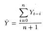
a) Moving Averages:
By this method we seek to ensure that the predicted value of a time series in a given period (month, quarter, year, etc.) is more or less equal to the average value of a time series in a number of past periods. For instance, with a three-year moving average, the forecasted value of the time series for the next period is equal to the average value of the time series in the last three periods.
Likewise, with a four-year moving average, the forecast for the next period is given by the average for the previous four periods, and so on.
The larger the number of years under consideration, the greater is likely to be the smoothing effect, inasmuch as less and less weights are attached to newer and newer observations. The greater the erratic or random component in the time series the more useful this technique proves to be.
The following table illustrates the method. It presents hypothetical data on the market share of a company in the last 12 years. A close look reveals that there is considerable random variation in the data, but there is hardly any secular or seasonal variation.

First we calculate three-year moving average, as shown in column (3). For example, the first value in col. (3) i.e., 21.67 for the fourth year is arrived at, by adding the first three values in col. (2) and dividing by (3) [i.e., 21.67 = (20+22+23)/3], If we have data for the first three years, our three-year forecast (F) for the fourth year would be 21.67. This has to be compared with the actual value of (A) i.e. 24 for the company’s market share in the fourth year.
In the next step we can drop the first-year observation in column (2) i.e., 20 and add the fourth observation, i.e., 24 and arrive at a new average, i.e., 23. This is the forecasted value of the company’s fifth-year market share.
This has to be compared with the company’s actual market share of 18 in Col. (2). If we proceed in a similar way, we can forecast the company’s market share,for the thirteenth year, i.e., 21.33. This is a genuine forecast because for this year no actual data were available.
On the contrary, by averaging the company’s market share in the first four years in column (2), we get the four-year moving average for- cast of 22.25 for the 5th year shown in Col. (5) of the table [i.e., (20 + 22 + 23 + 24) + 4 = 22.25].
This may be compared with the actual value of 18 in col. (2) The difference between the two (A-F) measures the magnitude of forecasting error, i.e., 4.25. From the above table moving average forecasts for other years may also obtained.
One time series model treats demand in the time series as interacting additively, i.e., if T is the trend, C the cycle, S the seasonal influences, and r the random shocks, then volume of sales is given as
Q = T + C + S + R
The four components may also appear in a multiplicative form like this:
Q = T x C x S x R
This formulation has the virtue that the effect of C, S, and R are proportional to the trend level of sales such that C, S and R are expressed as percentages of T.
Whatever the length of the forecast for which projection is to be used, one problem that immediately arises is to identify when persisting changes in the sales pattern have arisen, i.e., to distinguish from the behaviour of actual sales figures, a deviation from past behaviour that will continue into the period to be forecasted, from a deviation that will not.
In the longer-term case, for example as depicted in Fig. 12.4, to project the trend would suggest a sales level in 1991 of about 310,000. To project the cyclical curve would give a sales level of about 470,000 units. If the cycle follows its own past pattern and we have succeeded in identifying that pattern correctly, sales would be about 330,000 units.
Our problem is one of confidence that the actual sales figures for the year 1986 to the present, are part of the normal cyclical pattern and not a reflection of a persisting change in the trend.

In the shorter-term case, a sudden jump in sales over the last two months above the seasonal norm is likely to be a random event and sales next month may be expected to revert to the seasonal norm for that month, or it may bring into being a more long- lasting change.
In either case, the forecaster would not like his projection to reflect only the most recent sales figures. Some type of smoothing will be required. Otherwise, the forecasts will be widely erratic; but, on the contrary, one will not surely give a weight to sales figures occurring more distantly in time, equal to that accorded to that most recent figures.
Rather than use a simple moving average, therefore, one will probably use a weighting system. A common techniques used for the purpose is the ‘exponentially weighted moving average .
(b) Exponential Smoothing:
This technique is often used in conjunction with time-series analysis, especially when the trend and seasonal components in a time series are significant.
The basic methodology is like this:
If the forecaster has a time series (Yt, Yt-1,………. Yt-n) and seeks to obtain a forecast of Yt+1, he may hypothesize that the best forecast would be an average of previous values of Y. On the basis of this provisional statement or hypothesis, the forecaster has the following three options available.
1. He may use a simple mean of all the past data
so that the forecast of Yt+1 is equal to the average of the past N + 1 values of Y.
2. Alternatively he may use only some of the past data in calculating the simple average. In the extreme case, the forecaster may use only the previous value of Y so that Yt+1 = Yt.
3. Finally he may use weighted average of past observations, instead of using a simple average. In particular, the weighted average may be selected so that the most recent values of Y are given more weights than more remote observations.
An exponentially smoothed value derived from n periods of data may be expressed as


In this form the smoothed value in period f+1 equals a times the difference between the Y value for period f, plus the smoothed value in period t. Likewise the forecast value for period t+2 is given by Yt+1; that is Yt+2 = Yt+1
For cases in which a non-linear trend is present in a time series, it is convenient as to use quadratic or cubic smoothing.
Constant Growth Rate Projection:
The simple extrapolation model discussed above is based on the estimation of a constant absolute increase in sales in successive periods.
A common feature of the real world, however, is that sales tend to grow at a constant rate of change rather than at a constant absolute change. Thus, if sales of a particular product, say colour TV sets, grew at the rate of 5% per annum on the average over the last few years, we can then express the sales function as St = S0 (1+k)t,
where S0 is the sale of the base year, k is the average rate of growth of sales per annum and t is the number of periods after the initial period. If sales increased at the compound rate of k we could project sales for the future periods by inserting the appropriate values in the above equation. It may be noted that power functions may be transformed into linear forms by taking logarithms.
Therefore, the parameter of the above equation may be easily estimated using the least squares regression technique.
The Degree of Forecasting Accuracy:
One of the most important aspects of forecasting is ascertaining the degree of forecasting accuracy, i.e., testing the consistency of a forecast model with actual data.
In this context one may note that there are three ways of judging the forecasting reliability. The first approach in testing a model’s forecast capacity is to find out the correlation between forecast and actual values of variables. The simplest formula used for the purpose is
![]()
where σ f a is the covariance between the forecast and actual series, and σ f and σ a are the sample standard deviations of the forecast and actual series. A value of y very near to one or in excess of 0.99 is highly desirable. In cross-section analysis, this is a remote possibility because the important trend element in most economic data is held constant.
In such cases a value of 9.0 or 9.5 is considered satisfactory. Secondly, if we use the moving average method we can calculate the root mean square error (RMSE) of each forecast, and utilize the moving average that results in the smallest RMSE (weighted average error in the forecast).
The formula used for the purpose is:
![]()
where At is the actual value of the time series in period t, and Ft is the forecasted value and n is the total number of observations (the number of years in our example above). The forecast difference or the magnitude of error (i.e., A-F) is squared so as to “penalize larger errors proportionately more than smaller errors.”
In our last example the RMSE for the three- year moving average is
![]()
If this is found to be less than RMSE (not worked out here) for four-year moving average, then the three-year moving average forecast is considered better than the other one.
The predictive power of a model can be tested by considering this type of error. The smaller the value of this error the more confident we are about the forecast.