Monopoly Power: Degree, Sources and Measures | Markets

In this article we will discuss about:- 1. Meaning of Monopoly Power 2. Sources of Monopoly Power 3. Difficulties in Obtaining the Lerner Index 4. Measures of Monopoly Power under Price Discrimination 5. Concentration Ratios as Measures of Monopoly Power 6. The Herfindahl Index for Measuring Monopoly Power.

Meaning of Monopoly Power:

The monopolist is the only seller in the market of his product. As the only seller, he possesses a monopolistic dominance or monopoly power in the market. But the degree of monopoly power is not the same in the case of all monopolies. Generally speaking, the less elastic is the demand for a monopolist’s product, the more would be his degree of monopoly power, and vice versa.

That is, the degree of monopoly power depends upon the numerical coefficient (e) of the price-elasticity of demand for the monopolist’s product—a higher degree of monopoly power would be obtained at a smaller value of e and a lower degree of monopoly power at a larger value of e. This idea is supported by the formula given by Prof. A. P. Lerner (1903-82) for measuring the degree of monopoly power.

According to Prof. Lerner, degree of monopoly power in perfect competition is zero. At the equilibrium point of a competitive firm, we have p = AR = MR = MC, or p = MC, or p – MC = 0.

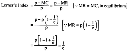
On the other hand, at the equilibrium point of a monopolistic firm, we have p = AR > MR = MC, or, p > MC, or, p – MC = positive. Prof. Lerner thinks that the larger the positive value of p – MC as a proportion of p, the larger would be the degree of monopoly power. Therefore, his formula for the degree of monopoly power is

Lerner’s Index of monopoly power = p – MC/p                          (11.48)

It is obvious from (11.48) that under perfect competition, the value of this index is zero (p – MC = 0), and in the case of monopoly, this index would be positive (p > MC).

We may now easily obtain the relation between the Lerner’s Index and the price-elasticity of demand for the product:

 

 

 

 

 

 

 

That is, the Lerner’s Index of monopoly power is nothing but the reciprocal of the numerical coefficient of price-elasticity of demand for the product, which supports our idea that the less elastic is the demand for the product, the more would be the degree of monopoly power, and vice versa.

We may easily understand the economic meaning of this idea. The smaller the price-elasticity of demand, i.e., the value of e, the smaller would be the response of demand for the product in response to a change in its price and the larger would be the power of the monopolist to charge a price in excess of MC, i.e., the larger would be value of p – MC and, therefore, of the Lerner’s Index.

Sources of Monopoly Power:

Monopoly power of a firm, is its ability to set the price of its product above the marginal cost. We have also seen that, in equilibrium, p – MC/p is equal to 1/e. This gives us that the smaller the price-elasticity of demand for the product the larger would be the monopoly power of the firm.

The main source of monopoly power, therefore, is the elasticity of demand for the product concerned. Now, the elasticity of demand for a firm’s product is determined by three factors.

These are:

(i) Elasticity of market demand,

(ii) The number of firms in the market, and

(iii) The nature of interaction among the firms.

(i) The Elasticity of Market Demand:

In the case of pure monopoly, there is only one firm that produces the product. Here, there is no difference between the elasticity of the firm’s demand and the elasticity of market demand. There­fore, in this case, the firm’s degree of monopoly power is determined directly by the elasticity of market demand for his product.

However, pure monopoly is rare in the real world. Because, barring exceptions, every product has at least a few close substitutes. In other words, in the real world we often find that a close substitute product-group is produced by a number of firms.

These firms compete over selling their respective products. In the case of each such firm, the elasticity of market demand for the product-group, hereafter called the ‘product’, provides the bottom line for the elasticity of its demand curve.

For example, if at any particular price, the e of the market demand for the ‘product’ be e* = 1.5 (say), then the e for the product of every firm would be at least 1.5. That is, if a firm decreases (or increases) the price of its product by 1 per cent, then the demand for its product would increase (or decrease) by at least 1.5 per cent.

(ii) The Number of Firms:

However, e for the product of a firm belonging to the group of firms that produce the ‘product’, may very well be more than the e* (here 1.5)—how much more would, of course, depend on the number of firms that produce the ‘product’. Let us see why.

If one among several firms producing the ‘product’, say, firm A, reduces its price by 1 per cent, say, the prices of the other firms remaining unchanged, then the product of A would become relatively cheaper and some of the customers of the other firms would switch over to A.

In this case, demand for the product of A would not only increase, in the first instance, by 1.5 per cent as given by the e* for the market demand for the product, but it would also increase somewhat more because of the ‘switch-over’ factor.

Similarly, if the price of the product of A increases by 1 per cent, then its demand would decrease not only by 1.5 per cent as given by e*, but it would also decrease somewhat more because of the ‘switch-over’ factor. For, now, the product of A would become relatively dearer and some of the customers of A would switch over to the close-substitute products of the group.

It is easy to understand from what we have said above that the larger the number of firms in the group, the more would be the strength of the ‘switch-over’ factor. That is, the larger the number of firms, the more would be the e for the product of A.

We may conclude then that the number of firms producing the ‘product’ is a determinant of the elasticity of demand for a firm’s product and the latter, in its turn, is a determinant of the degree of its monopoly power.

We may say then that the smaller (larger) the number of firms producing the close-substitute products, the smaller (larger) would be elasticity of demand for the product of a particular firm and the larger (smaller) would be the degree of its monopoly power (which is equal to 1/e)

We therefore have come, to an interesting conclusion that since in the case of pure mo­nopoly, the number of firms is only one, and since the e of the pure monopolist is equal to the bottom line e which is e*, the degree of monopoly power of a pure monopolist is the largest, i.e., it is larger than the monopoly power of a firm in a ‘non-pure’ monopolistic situation.

(iii) The Interaction among Firms:

If there are several firms producing the close-substitute products, called the ‘product’, then the monopoly power enjoyed by each of them would depend upon the interactions among them. If the firms compete aggressively, then they would undercut one another’s prices in order to increase their respective market shares.

Such aggressive competition among the firms may drive the prices of the products down nearly to the level of competitive price. In this case, p – MC would also be driven down and the degree of monopoly power of the firms would be relatively small.

On the other hand, the firms might decide not to compete among themselves, rather they might collude. In this case, collusion among the firms would restrict their outputs and increase their prices. So here they would have relatively high p – MC and the degree of their monopoly power would also be high.

Collusion may go to such a length that the firms may behave almost like one firm (giving rise to a multi-plant monopoly). In such a case, the degree of monopoly power would be the highest possible (approaching 1/e*).

We may conclude then that the monopoly power of a firm may arise from three sources.

These are:

(i) Elasticity of market demand for the product,

(ii) The number of firms, and

(iii) The nature of interaction among firms.

Difficulties in Obtaining the Lerner Index:

But there is some difficulty in obtaining the Lerner Index. For the elasticity of market demand for a ‘product’ is itself the elasticity of demand for the product of-a firm if there is only one firm producing the product, i.e., if there is a pure monopoly. But if the number of firms is more than one, then we have to infer the elasticity for each firm, which would depend on the elasticity for the product and the number of firms.

We would also obtain the Lerner Index if we knew the firm’s marginal cost, for in equilib­rium, MC itself is MR. But then the firm might hesitate to supply us the data about its MC. Therefore, here also, we may have to infer it from the monopolist’s behaviour. There are two ways to do this.

First, we may examine the periods when the industry was under competition. Since p = MC under competition, we might have some idea of the MC if we knew the price of the product. In the 19th century USA and Great Britain, this method of measuring monopoly power in the iron and steel industry has been used by the economists Peter Temin and Donald Mc Closkey.

Second, if the firm has a monopoly in the home market but it is a perfect competitor in the in the international market, then its profit-maximising condition gives us

MR_m = MR_C (= p_c) = MC                                     (11.49)

where MR_m = marginal revenue in the home or monopolistic market

MR_C = marginal revenue in the international or competitive market

p_c = price in the competitive market

MC = marginal cost of the firm

It is clear from above that the price of the product in the international market (p_c) would help us to know about the MC of the firm which is a monopolist at home. We may illustrate this with the help of Fig. 11.27. In Fig. 11.27, the MR curve of the monopolist in the home market is MR _m and the AR = MR curve (which is a horizontal straight line) in the international market is AR_C = MR_C at the level of the price, p_c, in this market.

Therefore, the combined MR curve or the horizontal sum of the MR_m and the MR_C curve would be the curve TEHS. The profit-maximising equilibrium of the firm would be obtained at the point H, where we would have

MR_m = MR_C = AR_C = p_c = MC                                   (11.50)

At the point H, total output sold by the firm is OL. Of this GL is sold in the international (competitive) market at the price p_c = HL, and OG is sold in the home (monopoly) market at the price p_m = DG. Marginal cost in both the markets is the same. It is HL = EG. Therefore, in Fig. 11.27, domestic sales is OG and the export sales is GL.

Let us now see what is the Lerner Index of monopoly power in this case. Since the MC for the total output is HL = EG and p_m = DG, the Lerner Index here would be DG- EG/DG = DE/DG. But if we consider only the home market, i.e., if we assume that there is no foreign market, then the equilibrium of the monopolist would have been given by MR = MC at the point B with p = AR and MR = MC equal to AC and BC, respectively.

The Lerner Index, in this case, would have been AB/AC. Since DE/DG is smaller than AB/AC (DE < AB and DG > AC), we have to come to the conclusion that the monopoly power would be smaller if the monopolist has to sell simultaneously in a competitive foreign market. This is what is expected.

For, over the foreign market part of the business, his monopoly power is zero. More objectively, the existence of the international market would make his total output larger which again would make his MC larger. In Fig. 11.27, for the home market output of OG his MC is FG, but for the total output his MC is much higher, it is HL—the higher the MC, the smaller would be the Lerner Index.

If there is a foreign market along with the home market, the proper measure of domestic monopoly power would be DF/DG, since FG is the MC of domestic output. But there is no way of inferring the marginal cost, FG, from the price ruling in the (competitive) foreign market.

It is clear from the above discussion that with the help of the price of the foreign market we may have a measure of the total monopoly power (TMP) of a firm who is a monopolist at home and perfect competitor abroad, and we have seen the difficulty with this measure which is less than the measure that might have been obtained if the firm were solely a monopolist.

The way out of this difficulty is to consider the total monopoly power (TMP) as approximately equal to the weighted average of the domestic monopoly power (DMP) and the foreign monopoly power (FMP) (which is zero), weighted by the respective sales, domestic and export, and then isolate the domestic monopoly power from the total monopoly power. We may do this in the following way. We have

 

 

 

 

 

 

 

 

 

 

 

 

 

 

 

 

 

 

 

 

 

 

 

 

 

 

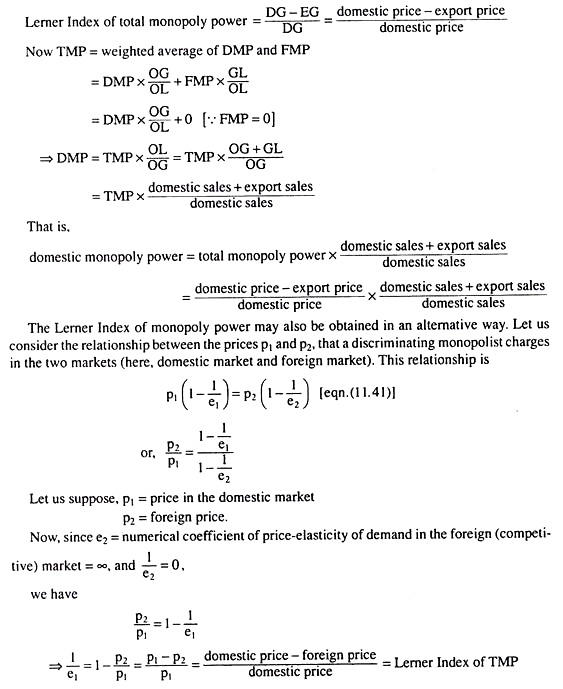
Therefore, the Lerner Index of (total) monopoly power is 1/e₁.

Measures of Monopoly Power under Price Discrimination:

Under price discrimination, the firm is able to discriminate between different markets in re­spect of the price of its product. This is proof enough that the firm possesses some monopoly power.

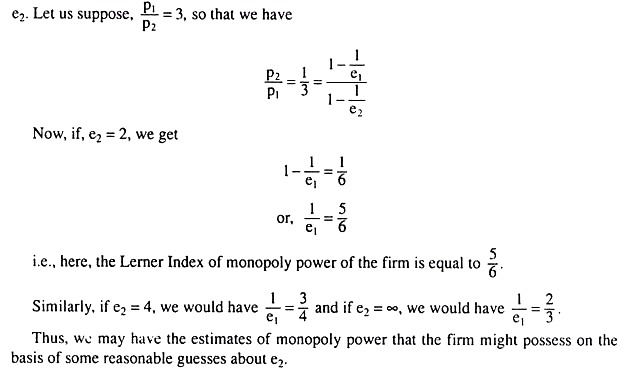
We have seen that if the monopolist practices price-discrimination in two markets, then the prices charged in the two markets, p₁ and p₂, are known to us. Now, if we know the elasticity of demand in only one of the markets, we may obtain a measure of monopoly power of the firm.

In the previous case, e₂ was known to be equal to ∞. But, if e₂ is not known to us exactly, then also, we may have an estimate of monopoly power on the basis of some assumptions about

Concentration Ratios as Measures of Monopoly Power:

In an industry, usually there exist some smaller firms and some larger firms in the sense that smaller firms have relatively smaller shares in total industry sales (or profits or assets), and the larger firms have relatively larger shares.

That is, sales (or profits or assets) may be more concentrated in a few firms of the industry, or such concentration may be less. Now, the size of the largest firms’ share in total industry sales, etc. is known as the concentration ratio.

For example, if we consider sales as the criterion, then the n largest firms’ share in total industry sales is called an n-firm concentration ratio which is denoted by CR_n. Usually, the four firm and eight firm concentration ratios denoted by CR₄ and CR₈, are used as a measure of monopoly power.

The concentration ratio may act as a measure of monopoly power because in a competi­tive industry, sales are more evenly distributed among firms—concentration of sales is more or less absent. On the other hand, in a monopolistic industry, sales tend to concentrate in a few large firms—in the limiting case, sales are concentrated in only one firm when we have the case of a pure monopoly.

Let us suppose that there are five firms in an industry, and the shares of the firms arranged in a descending order are as follows:

We can compute the cumulative shares for the n largest firms for n = 1, 2, 3, 4, 5.

These cumulative shares are:

We have obtained above that the cumulative share of the first two largest firms (CR₂) is 0.80. Similarly, CR₃ = 0.90, CR₄ = 0.96 and CR₅ = 1.00. If we plot the cumulative percentage of sales against the cumulative number of firms from largest to smallest, we would obtain a curve called the concentration curve. The concentration curves of three typical industries have been shown in Fig. 11.28.

The figure shows us that concentration is larger in industry A than in the industries B and C. But whether concentration is larger in B or C depends on whether we are comparing the concentrations in the largest four firms (CR₄) or in the largest eight firms (CR₈).

If we look at CR₄, concentration is larger in industry B, but if we look at CR₈, concen­tration is larger in industry C. This is the basic defect of concentration ratios as measures of monopoly power.

There may be another problem also with the concentration ratios. From the point of view of sales, one industry may be more concentrated than another and, from the point of view of profits or assets the latter may be more concentrated than the former.

A third problem with the concentration ratio is that it does not take into account the number of firms. For example, in the example of five firms we have obtained CR₄ = 0.96. In another industry with 100 firms the CR₄ may also be obtained to be 0.96. We cannot really compare the monopoly power or the competitiveness in these two industries, since the numbers of firms in the two cases are different.

A fourth problem with the concentration ratios is that they are usually based on the distribu­tion of firms in the domestic industry and they completely ignore the picture in the foreign sector. Yet the existence of foreign competition might considerably affect the behaviour of the domestic firms.

The Herfindahl Index for Measuring Monopoly Power:

The Herfindahl Index (named after Orris C. Herfindahl) avoids some of the major problems involving the use of concentration ratios (CRs).

This index is denoted by HI and defined as:

where n is the number of firms in the industry and S; is the market share of the ith firm (i = 1,2, …, n). As is evident, this index reflects both the number of firms and their relative sizes. For, the example we have already considered, HI to be obtained would be

HI = (0.50)² + (0.30)² + (0.10)² + (0.06)² + (0.04)² = 0.3552.

In case all the firms had equal market shares of 0.2, the Herfindahl Index would be

HI = 5 (0.2)² = 1/5

That is, if there are n firms in an industry all having equal shares, the share of each firm would be 1/n and we would have

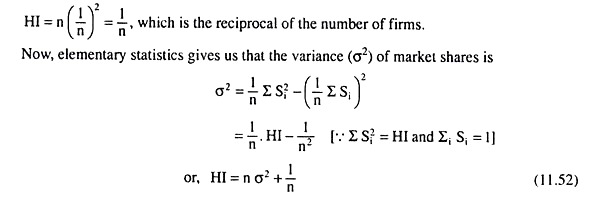
Thus, HI depends solely on two things, viz., the variance of the market shares and the number of firms. If the market share is equally distributed among the firms, i.e., if σ² = 0, the measure of monopoly power which is given by the HI, would assume the value 1/n, and this is also the minimum value of the HI (^._.^. σ² ≥ 0) for a given n.

Therefore, if there are many firms in the industry that are more or less of equal size, the value of HI would be small, since n is large and σ² is close to zero. On the other hand, if n = 1, then we would have σ² = 0, and in that case the HI would be equal to 1.

In other words, in the case of pure mo­nopoly, the HI would be equal to 1, and it is the maximum value of HI. That is, we have obtained that the HI would lie between and 1, both ends inclusive (1/n ≤ HI ≤ 1), and a larger HI indicates a greater monopoly power.