8 Important Pricing Strategies Adopted by Firms

The following points highlight the eight important pricing strategies adopted by firms.

The strategies are: 1. Pricing a New Product 2. Multiple Products 3. Product-Line Pricing 4. Pricing over the Life Cycle of a Product 5. Cyclical Pricing 6. Transfer Pricing 7. Differential Pricing 8. Cost-Plus or Full-Cost Pricing.

Strategy # 1. Pricing a New Product:

Pricing is a crucial managerial decision. Most companies do not encounter it in a major way on a day-to-day basis. But there is need to follow certain additional guidelines in the pricing of the new product. The marketing of a new product poses a problem for any firm because new products have no past information.

Here the firm is also not in a position to determine consumer reaction. The question is, what do we mean by a new product? New products for our purposes will include original products, improved products, modified products and new brands that the firm develops through its own R&D efforts.

When fixing the first price, the decision is obviously a major one. When the company introduces its product for the first time, the whole future depends heavily on the soundness of initial pricing decision.

Top management is accountable for the new product’s success record. Top management must establish specific criteria for acceptance of new product ideas especially in a large multidivisional company where all kinds of projects bubble up as favourites of various managers.

There are always competitors who would also like to produce it at the earliest opportunity. Pricing decision assumes special importance when one or more competitors change their prices or products or both.

Sometimes, the competitors may introduce a new brand without altering the price of an existing brand. If the new brand is perceived to compete with a given brand more effectively, then the firm in question may have to think on its pricing policy once again.

The price fixed for the new product must:

(i) Earn good profits for the firm over the life of the product;

(ii) Provide better quality at a cheaper price and at a faster speed than competitors;

(iii) Face rising R&D, manufacturing and marketing costs, and

(iv) Satisfy public criteria such as consumer safety and ecological compatibility.

The firm can select two types of strategy:

(A) Skimming Pricing.

(B) Penetration Pricing.

(A) Skimming Pricing:

Skimming pricing is known as charging high price in initial stages. This can be followed by a firm by charging skimming price for a new product in pioneering stage. When demand is either unknown or more inelastic at this stage, market is divided into segments on the basis of different degree of elasticity of demand of different consumers.

This is a short period device for pricing. The demand for new products is likely to be less price elastic in the early stages, that is, the initial high price helps to “Skim the Cream” of the market which is relatively insensitive to price.

This policy is shown in Fig. 1, where the manu­facturer of new product initially determines OP price and sells OQ quantity. Thus he receives KPMN abnor­mal profit. Under this policy, consumers are distin­guished by the producers on the basis of their intensity of desire for a commodity.

For example, in the begin­ning the prices of computers, TVs, electronic calcula­tors, etc., were very high but now they are declining every year. A high initial price together with heavy pro­motional expenditure may be used to launch a new prod­uct if conditions are appropriate.

These conditions are listed below:

(i) Demand is likely to be less price elastic in the early stages than later. The cross elasticity demand should be very low.

(ii) Launching a new product with a high price is an efficient device for breaking the market into segments that differ in price elasticity of demand.

(iii) When the demand elasticity is unknown, high introductory price serves as a refusal price during the stage of exploration.

(iv) High initial prices help to finance the floatation of the product. In the early stages, the cost of production and organisation of distribution are high. In addition, research and promotional investments have to be made.

(B) Penetration Pricing:

Penetration price is known as charging lowest price for the new product. This is aimed to quick in sales, capture market share, utilise full capacity and economies of scale in productive process and keep the competitors away from the market.

Penetration price policy can be adopted in the following circumstances:

(i) There is very high price elasticity of demand.

(ii) There are substantial cost savings due to enhanced production process.

(iii) By nature the product is acceptable to the mass of consumers.

(iv) There is no strong patent protection.

(v) There is imminent threat of potential competition so that a big share of the market must be captured quickly.

Penetration price is a long term pricing strategy and should be adopted with great caution. Penetra­tion pricing is successful also when there is no elite market. When a firm adopts a penetrating pricing policy, adjustments to price throughout the product life cycle are minimal. Since this policy prevents competition, it is also referred to as ‘Stay-out’ price policy.

Penetration price is explained in Fig. 2, where market price is OP₀, and quantity demanded is OQ₀. Now the producer of a new product fixes the price less than the market price i.e., OP₁ and sells OQ₁ more quantity. Obviously, it has a wide potential market.

The comparison between skimming pricing and pen­etration pricing is that high skimming price policy needs vigorous and costly promotional effort to back it but low penetration price would require low promotional expendi­tures.

But the policy is inappropriate where:

(i) The total market is expected to stay small, and

(ii) The new product calls for capital recovery over a long period.

Strategy # 2. Multiple Products:

The traditional theory of price determination is based on the assumption that the firm produces a single homogeneous product. But firms usually produce more than one product. When firms produce several products, managers must consider the interrelationships between those products.

Such prod­ucts may be joint products or multi-products. Joint products are those where inputs are common in productive process. Multi-products, are creation of the product line activity with independent inputs but common overhead expenses. Pricing of multi-product or joint product requires little extra caution and care.

For evolving price policy for multi-product firm, certain basic considerations involved in decision making are:

(i) Price and cost relationship in product line,

(ii) Demand relationship in product line, and

(iii) Competitive differences.

They are explained as follows:

(i) Price and Cost Relationship:

For evolving a price policy for any product, price and cost relationship is the basic consideration. Cost conditions determine price. Therefore, cost estimates should be correctly made. Although a firm must recover its common costs, it is not necessary that prices of each product be high enough to cover an arbitrarily apportioned share of common costs.

Proper pricing does require, however, that prices at least cover the incremental cost of producing each good. Incre­mental costs are additional costs that would not be incurred if the product were not produced.

As long as the price of a product exceeds its incremental costs, the firm can increase total profit by supplying that product. Hence decisions should be based on an evaluation of incremental costs. A price that offers maximum contribution over costs is generally acceptable but in multi-product cases, incremental cost becomes more essential to make such decisions.

A set of alternative price policies should be considered and they are:

(i) Prices of multi-products may be proportional to full cost. This price may produce equal percent­age of profit margin for all products. If the full cost for all products are assumed equal then the pricing will be equal.

(ii) Pricing for multi-products may be proportional to incremental cost.

(iii) Prices of multi-products may be assessed with reference to their contribution margin as proportional to conversion cost.

(iv) Prices of multi-product may be fixed differently keeping into consideration market segments.

(v) Prices for multi-products may be fixed as per the product life cycle of each product.

(ii) Inter-relation of Demand for Multi-product:

Demand inter-relationships arise because of competition in which case they become substitutes or they may be complementary goods. Sale of one product may affect the sale of another product. Different demand elasticity of different consumers may allow the firm to follow policies of price discrimination in different market segments. Two products of the same price may be substitutes to each other with cross elasticity of demand due to high degree of competitiveness.

In such a situation, pricing of the multi-products will have to be done in such a long way that maximum return could be obtained from each market segments by selling maximum products. Demand inter-relationships in the case of multiple products make it clear that we should take into account a thorough analysis of the total effect of the decision on the firm’s revenues.

(iii) Competitive Differences:

Yet another important point should be considered for making price decisions, for a product line is the assessment of degree of competitiveness. Such an assessment will set up market share for each product. A product having large market share can stand a high mark­up and can contribute to bear the losses.

There is competition among a few sellers of a relatively homogeneous product that has enough cross elasticity of demand so that each seller must in his pricing decisions take account of rivals’ reaction. Each producer is actually aware of the disastrous effects that an announced reduction of his own price would have on the prices charged by competitors. The firm should also analyse whether the competitors have free entry to the market or not.

Marginal Technique for Pricing Multi-products:

Marginal technique for pricing multi-products is based on the logic that when the firm has spare capacity, unutilised technical resources, managerial and organisational abilities and capabilities, the firm enters into production of various other products with most profitable uses of alternatives. The product is technically independent in the production process. For selecting these alternatives, the firm considers marginal costs of each such alternative and adopts those which offer higher margin on cost through sales.

Since each additional unit produced entails an additional cost as well as generates additional rev­enue, the logic of profit maximisation stresses that production should be stabilised at a point where MR just covers MC. Marginal cost more accurately reflects those changes in costs which result from a decision. Marginal pricing is more useful because of the prevalence of multi-product firms.

A firm shall produce the multi-product to the level where MR from sales of all these products equals the MC. If MC is more than MR then the firm shall stop producing and selling one of the products which offer less MR than MC.

Pricing of Multiple Products or Joint Products:

Products can be related in production as well as demand. One type of production interdependency exists when goods are jointly produced in fixed proportions. The process of producing mutton and hides in a slaughter house is a good example of fixed proportion in production. Each carcass provides a certain amount of mutton and hide.

There is little that the slaughter house can do to alter the proportion of the two products. When goods are produced in fixed proportion they should be thought of as a ‘product package’. Because there is no way to produce one part of this package without also producing the other part, there is no conceptual basis for allocating total production costs between the two goods.

Pricing of joint products can be explained under two different circumstances:

(i) When there is fixed proportion of products.

(ii) When there is variable proportion of products.

(i) Joint Products with Fixed Proportion:

In joint product case with fixed proportion of quantity, there is no possibility of increasing one at the expense of another. In this situation, the costs are joint and cannot be increased at the expense of another. In this situation, the costs are joint and cannot be allocated to each product on any sound basis. Although the two goods are produced together, their demands are independent.

However, there is a single marginal cost curve for both products. This reflects the fixed proportion of production, i.e., the marginal cost is the cost of supplying one more unit of the product package. Where goods are jointly produced as in the case of mutton and hides, pricing decision should take this interdependency into account.

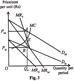
Figure 3 indicates how profit maximising prices and quantities are determined. P_M and P_H represent the most profitable prices for the joint products.

The figure carries the assumption that each product is produced in fixed proportion because the output point for both is one and the same whereas their demand and marginal revenue curves are separate for different markets existing for them. MR_M and MR_H are the marginal revenue curves for mutton and hides respectively. But when an addi­tional animal is processed at a slaughter house both mut­ton and hide become available for sale.

Hence the mar­ginal revenue associated with sale of a unit of the prod­uct package is the sum of the marginal revenues. This sum is represented by the line MR_T. MR_T is determined by adding MR_M and MR_H for each rate of output.

Graphically, it is the vertical sum of the marginal revenue curves of the two products. The profit maximising output Q_O is determined by the intersection of MR_T and MC curve at point E with price of mutton OP_M and of hides OP_H.

(ii) Joint Products with Variable Proportions:

Pricing of joint products which can be produced with variable proportions presents interesting analysis of price, cost and output. When it is possible for a firm to produce joint products in different proportions, the total cost has to be divided among different products because there cannot be a single marginal cost curve.

Figure 4 illustrates the pricing method of multiple products with variable propor­tions wherein three main things are to be observed:

(i) The production possibility curve is concave to the origin indicating imperfect adaptability of productive resources in producing products A and B. In other words, it indicates the quantity of A and B which can be produced with the same total cost. It is the isocost curve labeled as TC in the figure.

(ii) The iso-revenue lines define the prices which the firm receives for the two products irrespec­tive of any combination of their output. They are shown as TR in the figure.

(iii) The best combinations are the points of tangency of isocost curves and isorevenue lines for optimum production and maximisation of sales revenues or profits.

Thus the optimal output combination is at a point where an isorevenue line is tangent to an isocost curve. We can find the optimal combination by comparing the profit level at each tangency point and choosing the point with the highest profit level, given fixed product prices.

Suppose a firm produces and sells two products A and B, given their prices. Each isocost curve, TC, shows the quantities of these products that can be produced at the same cost. Each isorevenue line shows the combinations of outputs of A and B that yield the same revenue.

The problem facing the firm is to determine the outputs of joint products A and B. To solve it, let us start with an output combination where an isorevenue line is not tangent to the isocost curve. Let us take such a point as P in the figure. This cannot be the optimal output combination because it is possible to increase revenue without changing cost by moving to point R on the same isocost curve where the isorevenue line is tangent to the isocost curve.

Besides, the firm has to take into consideration the profit maximisation optimal output of combina­tion A and B products. For this, it compares the level of profit at each tangency point and chooses that point where the profit level is the highest.

In the figure, there are four tangency points K, R, S and T corresponding to the profit levels π = Rs 2 crore, π = Rs, 4 crore, π = Rs 6 crore and π = Rs 4 crore respectively. It is clear from the above that the firm will choose the optimal output combination at point S where it produces and sells OA₃ units of product A and OB₃ units of product B and earns the highest profit Rs. 6 crore. It cannot produce at the higher output combination point T as compared to S because its profit level will fall to Rs 4 crore.

Strategy # 3. Product-Line Pricing:

Product line pricing is an important practical problem for most modern industrial enterprises. Since almost every firm makes several related products, product line pricing is an important phase of price policy.

Product line pricing refers to the determination of prices of the individual products which form units of an output package. From the viewpoint of management a typical modern firm produces multiple models, styles or sizes of output each of which can be considered a separate product.

Although product line pricing requires same economic concepts used for single product pricing, the analysis becomes complicated, however, by demand and production externalities which arise because of substitutability or complementary between the products on the demand or the production side.

The problem of product line pricing is to find the proper relationship among the prices of mem­bers of a product group. Product line pricing can include use-differentials (e.g., fluid milk vs. cheese milk), seasonal differentials (e.g., morning movie specials) and style cycle differentials.

These are all phases of product line pricing. Our analysis of product line pricing is divided into two parts, the first sets forth a general approach to the problem; and the second applies this approach to some specific cases.

General Approach:

We discuss, in this section, problems of exploring demand relationships and competitive differ­ences and of making and using cost estimates for pricing related products.

Alternative Policies of Price Relationship:

A logical approach to product line pricing is to start with a picture of the alternative kinds of policy regarding the relationships among prices of members of a product line.

Let us examine some systematic patterns below:

(i) Prices that are Proportional to Full Cost:

Prices that are proportional to full cost, i.e., that produce the same percentage net profit margin for all products. Here cost plus pricing is followed.

(ii) Prices that are Proportional to Incremental Costs:

Prices that are proportional to incre­mental costs i.e., that produce the same percentage contribution margin over incremental costs for all products. Incremental cost is the additional cost of added units.

(iii) Prices with Profit Margins that are Proportional to Conversion Cost:

Prices with profit margins that are proportional to conversion cost, i.e., that take no account of purchased materials cost. Conversion costs refer to costs incurred to convert the raw materials into finished products.

(iv) Prices that produce Contribution Margins that depend upon the Elasticity of Demand:

Buyers with high incomes are usually less sensitive to price than those that make up the mass market and it is often profitable to put higher profit margins as products for the plushy-class markets than for the rough and tumble mass markets.

(v) Prices that are systematically related to the Stage of Market and Competitive Develop­ment of Individual Members of the Product Line:

Many products pass through life cycles. A product line pricing policy that specifically recognises that a company’s various products are at different stages in their life cycles and hence face different market acceptance and competitive intensity has much to command it. This method emphasises that the firm should charge high price for those products in the line which are in their pioneering stage and prices are kept low for products in the maturity stage.

Competitive Differences:

An analysis of competition is frequently a vital phase of product line pricing because differences of competitive selling among products call for differences in profit margins or distribution margins.

Even though it is not possible to measure the relevant aspect of competitive differences among products. Differences in competitive condition depend upon the firm’s share of each product in the market. Here two aspects of competition, existing and potential, have to be considered.

Existing competition can be measured indirectly by several of its symptoms:

(i) The number of competitors,

(ii) The market share, and

(iii) The degree of similarity of the competitive products.

In general, the fewer the competing sellers, the higher the margins, aside from other dimensions of competition. A product with a dominant market share can stand a higher mark-up since the presumption is that it has competitive superiority. The degree of similarity of the competitive product indicates that differentiated or unique products can have higher prices.

Potential competition can use indices like:

(i) Incentives for competitive entry,

(ii) Patent barriers,

(iii) Financial barriers, and

(iv) Technological barriers.

Existing profits of the firm are the index to the entry of other firms. Higher profits will attract other firms. Patent barriers to future competition depend upon the ability to initiate the production process. Financial barriers can be quantified by guessing how much money it would require to develop a com­petitive product and sell it. Technical barriers are similar to patent barriers.

Cost Estimates:

The cost should be the dominant if not the sole consideration in determining the relationship of prices within a product line. Cost estimates are indispensable for accurate analysis of almost every kind of pricing problems. Cost estimates are needed in product line pricing to project roughly the effects upon profits of different price structures.

Specific Problems:

Other dimensions that have to be considered in the philosophy of products line pricing are:

(i) Pricing products that differ in size.

(ii) Pricing products that differ in quality.

(iii) Charm prices.

(iv) Pricing special designs.

(v) Load factor price differentials.

(vi) Pricing repair path.

(vii) Pricing leases and licenses.

They are explained as under:

(i) Pricing Product that differ in Size:

The intensity of competition often varies with size. The logical role for size as a pricing criterion is as a measure of value of the buyer. In selecting the pattern of relationship of price to size, much depends upon whether the typical buyer has freedom to substitute one size of product for another. The best example of size-differential pricing problems is given with reference to fractional page advertising rate in newspapers.

(ii) Pricing Products that differ in Quality:

The pricing decision here depends primarily upon the strategic objectives of having products that differ in quality. Sometimes the purpose of high quality items is to bring prestige to the entire line. The firm may also produce products of lower quality to compete with the low priced product in the market. The low quality products are introduced at low prices to face competition.

(iii) Charm Prices:

Charm price theory is based upon consumer psychology that prices ending in odd figures e.g., Rs. 4.95 and Rs. 9.95 have greater effect than odd or even prices such as Rs. 5 and Rs.10. This is a point of controversy and empirical research, yet it does not permit a conclusive answer. Newspaper advertisements are dominated by prices ending in odd numbers. Another explanation is that odd figures convey the notion of a discount or bargain.

(iv) Pricing Special Designs:

Pricing special designs is a common practice to estimate normal full cost, then add to cost a fixed percentage to represent a fair or desirable profit. The price decision as special order is really a decision as to whether or not to produce the product at all. Here cost plays a peculiar role in special order pricing. An important base for special order pricing is good judgment in estimating accurately the future cost of unfamiliar products.

(v) Load Factor Price Differentials:

Here firms charging different prices at different times for the same product or service in order to improve the sellers’ load factor have important profit potentiali­ties for many producers. Such load factor price differentials are part of peak load pricing theory.

Examples of load factor price differentials are off peak rates for electric energy, morning movies, summer discounts on winter clothing, etc. It need not be for the same product at different period. Analysis of demand, cost and competition should enter into this consideration.

(vi) Pricing Repair Parts:

All producers of durable goods face the problems of pricing the repair parts or spare parts. Some firms even experience higher sales receipts from repair parts production than from new equipment. Spare parts pricing has an element of monopoly.

This monopoly power is, how­ever, always restricted by competition of various forms. Pricing of spare parts should not be related to relative average cost or to relative weight. Parts that are readily available should be sold at relatively low prices. Parts that the buyer can himself rebuild or get it made, for them prices should be low.

(vii) Pricing Leases and Licenses:

Royalty licensing and leasing of capital goods and patents reflect application of market segmentation pricing. Uniform price cannot be charged. The price charged on these is closely related to the benefits the firm receives. This pricing practice reaps for the seller a share of the gains of the most advantageous users.

Benefits are determined by the purpose for which the equipment is obtained, the rate of utilisation, the efficiency of alternatives and so forth. As far as royalty price is concerned, it need not consider the development costs that were incurred in creating the equip­ment.

Strategy # 4. Pricing over the Life Cycle of a Product:

The cycle begins with the invention of the new product. The innovation of a new product and its degeneration to a common product is termed as the life cycle of a product. It is an important concept in marketing that provides insights into a product’s competitive dynamics. The life cycle of a product portrays distinct stages in the sales history of a product.

Corresponding to these stages are distinct opportunities and problems with respect to market strategy and profit potential. By identifying the stage that a product is in, or may be headed toward, companies can formulate better marketing plans. Figure 5 depicts the life cycle of a product.

Every product moves through a life cycle having five phases as shown in the figure and they are:

(i) Introduction:

This is the first stage in the life cycle of a product. This is an in­fant stage. The product is a new one. The product is put on the market, awareness and acceptance are minimal. There are high pro­motional costs. Therefore, the profit may be low. The firm can use two types of pric­ing policy, i.e., skimming price policy or centralising price policy in this stage.

(ii) Growth:

In this stage, a product gains acceptance on the part of consumers and businessmen. The product begins to make rapid sales gains because of the cumulative effects of introductory promotion, distribution work or mouth influence. The product satisfies the market. For the purpose of pricing, there is not much difference between growth and maturity stages.

(iii) Maturity:

At this stage, keen competition increases. Sales growth continues, but at a dimin­ishing rate, because of the declining number of potential customers. Competitors go for mark-down price. Additional expenses are involved in the product’s modification and improvement, thus profit margin slips. This period is useful because it gives out signals for taking precaution in pricing policy.

(iv) Saturation:

In this stage, the sales are at the peak and further increase is not possible. The demand for the product is stable. The rise and fall of sale depend upon supply and demand. There is little additional demand to be stimulated, it happens to be its replacement demand. Therefore, the product pricing in the saturation stage is full cost plus normal mark-up.

(v) Decline:

Sales begin to diminish absolutely as the customers begin to tire of a product. The competitors have entered the market with substitutes and imitations. Price becomes the competitive weapon. The product should be reformulated to suit the consumers preferences, it is possible in the case of few commodities.

Throughout the cycle, changes take place in price and promotional elasticity of demand as also in the production and distribution costs of the product. Therefore, pricing policy must be adjusted over the various phases of the cycle.

Strategy # 5. Cyclical Pricing:

Cyclical pricing refers to the pricing decisions of the firm which are taken to suit the fluctuations in the business conditions. To simplify decision making in response to the alterations in the entire economic system, it is necessary for the firm to have some kind of policy based on cyclical price behaviour. It is more apparent to say that prices are slashed during recession and pegged up during a demand-pull or a demand-push.

In formulating a policy of cyclical pricing, various factors such as demand, competition, cost- push, price rigidity, price fluctuations, fluctuations due to substitutes, purchasing power, market share and demand fluctuation should be taken into account.

They are explained as under:

(i) Demand:

The commodities are divided into durable and non-durable goods. The necessaries fall under non-durable goods and demand for them is constant and inelastic. The purchase of necessary- goods cannot be postponed but the purchase of durable goods can, however, be postponed. Under imperfect market conditions, demand plays an important role.

(ii) Competition:

If the market is imperfect, firms compete against each other and there is an element of interdependence. A policy change on the part of one firm will have immediate effects on competitors. Price cuts lead to price war. Therefore, adjustments have to be made.

(iii) Cost-push:

Producers tend to pass on increase in cost of production to consumers in the form of higher prices.

This may happen due to:

(a) Wage increases higher than output;

(b) Inadequate investment in plant may reduce output;

(c) Shortages of factors of production; and

(d) Increase in price of basic raw materials.

In these conditions costs are bound to rise. Under this situation, what kind of pricing policy should be followed by the firms? It is difficult to answer this question.

Joel Dean suggests that in formulating a policy of cyclical prices, the following factors may be considered:

(a) Price Rigidity:

Firms do not believe that prices change because of business cycles. The cyclical fluctuations are caused by economic factors like income, profit and psychological factors like expectations of the consumers. They have control over these factors. They are also of the opinion that it is not healthy to change prices in response to cyclical fluctuations.

(b) Price Fluctuation:

Price fluctuations conform to cost changes at current full cost, standard full cost, and incremental cost. Confirming cyclical changes in prices to changes in company costs is another popular cyclical policy. It amounts to stabilising some sort of unit profit margin.

(c) Fluctuation due to Substitutes:

The use of substitute product as a cyclical pricing guide is an appropriate price policy in many situations. It may also stabilise the industry’s share of the vast substi­tute market.

(d) Purchasing Power:

If prices can be reduced because of a fall in the purchasing power of the people during a depression, then we have what is known as the blanket index of the purchasing power. Purchasing power index is only an average that covers up great disparities. Therefore component prices are more important.

(e) Market Share:

Market share is determined by many factors and price is an important deter­minant. Price policy has a profound effect upon the larger share of the substitute market. A reduction in price would increase the market share. Market share can be a useful pricing guide for cyclical pricing.

(f) Demand Fluctuations:

If there are shifts in demand, they should be taken into account in setting prices. They are more important than the elasticity of demand. One recession pricing policy is to change prices in relationship to some appropriate index of shifts in demand for the product.

This pricing method assumes:

(i) That flexible rather than rigid prices are appropriate,

(ii) That changes in prices in the past have adjusted for changes in demand correctly,

(iii) That these past pricing objectives are today’s objectives, and

(iv) That cost behaviour and competitive reactions will be the same as in similar periods in the past.

Strategy # 6. Transfer Pricing:

Transfer pricing is one of the most complex problems in pricing. The growth of large scale multi- divisional organisations has given rise to the problem of pricing commodities that are transferred inter­nally from one division to another.

The divisional organisations are preferred due to the following reasons:

(i) It provides a systematic way of delegation and decision making

(ii) For proper evaluation of contribution, and

(iii) For the precise evaluation of manager’s performance.

This involves the problem of sub-optimisation.

The transfer price must satisfy the following two criteria:

(i) It should help establish the profitability of each division or department.

(ii) It should permit and encourage maximisation of the profits of the company as a whole.

For determining the transfer price there are three alternative methods.

They are explained as follows:

(i) Market Price Basis:

The suitable system of transfer of goods from one division to another under the same management to another company, is the market price basis. The market price should be the transfer price. Wherever a market price exists for a product, the inter-divisional transfer price should equal the market price to avoid sub-optimization. This method definitely avoids the possibility of passing the inefficiencies of one department to the other departments.

(ii) Cost Basis:

In case the product produced by a division of the firm can be sold only to another division of the firm, the inter-divisional transfer should be priced at the level of the actual cost of production. Here transfer prices will be useful to achieve the best joint level of output. It will maximise profits.

(iii) Cost Plus Basis:

Under this method the goods and services of each department are charged on the basis of actual cost plus a margin by way of profit. The major defect of this method is that the transferring department may add a high margin so as to raise the profit of the department. It may result in setting the ultimate price unduly high thereby affecting sales.

Transfer Price Determination:

Firms have the following objectives while determining the transfer price:

1. The aim of the firm is to ensure that its goal coincides with that of the related divisions.

2. The price of the transferred product should be so determined that the profitability of each division could be ensured.

3. The price should be such that it could induce profit-maximisation of the company as a whole rather than of a particular division.

Large firms often divide their operations into various divisions or departments. One division uses the product of the other division. In such a situation, firms are faced with the problem of determining an appropriate price for the product transferred from one division or sub-division to the other.

In other words, transfer pricing refers to the price determination of goods and services transferred among interdependent units or divisions within the organisation. This operates as a measure of the economic achievements of profit making divisions in the organisation. It is necessary to consider various situa­tions while determining transfer price.

1. Transfer Pricing: Absence of an External Market:

If an intermediate product has no external market, transfer pricing will be according to the mar­ginal cost of the producer.

Suppose that a firm has two independent divisions production division and marketing division. The Production division produces one product that is sold to the marketing division of the same firm. The price at which it sells is called transfer price. Further, the marketing division presents that product as a final product by packaging it and sells it to the public.

We also assume that the product manufac­tured by the production division has no market outside the firm. In other words, the marketing division completely depends upon the production division for the supply of the product and the production division depends on the marketing division for its demand. Therefore, the total quantity of the product manufactured by the production division must be equal to the amount sold by the marketing division.

In Fig. 6  MC_p and MC_M are the cost curves of production division and marketing division respec­tively and MC is the firm’s cost curve. This curve is the summation of MC_P and MC_M curves. D_F is the firm’s demand curve and MR is the marginal revenue curve for the final product. The firm will be in equilib­rium at point E where its MC curve cuts its MR curve. The firm will be selling OQ quantity of the product at OP price.

Now, the question is how much price the produc­tion division should charge for its product from the mar­keting division? The transfer price is equal to the mar­ginal revenue of the production division. The transfer price once determined is always stable because the de­mand curve of production division is horizontal on which the marginal revenue of production division is equal to the transfer price, i.e., D=MR_p=P₁.

The production divi­sion will earn the maximum profit for its intermediate product at that point where the transfer price (P₁) which is also its marginal revenue (MR_P), is equal to its marginal cost (MC_p), i.e., P₁=MR_P=MC_p. This situation is at E₁ point where the MC_p curve cuts the. D=MR_P=P₁ curve from below.

2. Transfer Pricing: Presence of an External Market:

If there is an external market for the intermediate product, the production division may produce more product than the marketing division needs and may sell the surplus product in the external market. On the other hand, it may produce less than the needs of the marketing division and the marketing division can obtain the rest of its requirements from the external market. Thus, it is more free for maximising its profit.

(1) Transfer Pricing:

In a Perfectly Competitive External Market In the case of a perfectly competitive external market, where the intermediate product can be sold or bought from the perfectly competitive outside market by the firm, the quantity produced by the production division may not be equal to the required quantity for the marketing division.

In such a situation transfer price of intermedi­ate product is the market price of that product. The firm can be in the maximum profit situa­tion only when all its divisions operate at their related MR = MC points. In these conditions, we explain transfer pricing in terms of Figure 7.

In the figure, D is the demand curve of intermediate product which is a horizontal line. This curve shows marginal revenue (MR_p), average revenue (AR_p) and price (P) of the pro­duction division.

According to the figure, the production division will receive the maximum profit at OQ₂ output level because at this level marginal cost of production (MC_p) is equal to its marginal revenue (MR_p) which determines OP₁ price. Here the equilibrium is at point E where the MC_p curve cuts the D=AR_p = MR_p curve from below.

To maximise total profit of the firm in the perfectly competitive market, it will be appropriate to keep transfer price at OP₁ level. It is at this price that the production division will sell its intermediate product to the marketing division or to outside customers, and the marketing division will also give only OP₁ price for the intermediate product to the production division.

The marginal cost curve of the marketing division is MC_M which is the summation of marginal marketing cost and transfer price P₁. To maximise its profit, marketing division will have to purchase OQ₁ quantity where its marginal cost MC_M is equal to its marginal revenue MR_M at point E₁.

In the figure, the maximum profitable quantity for the production division will be OQ₂ and that for the market­ing division OQ₁. Hence, the production division will sell OQ₂– OQ₁ = Q₂Q₁ portion of its output in the external market.

(2) Transfer Pricing: In Imperfectly Competitive External Market:

Here we discuss trans­fer pricing in that market situation where the production division sells its product in imperfectly com­petitive external market as well as to the marketing division. In such a situation, an important problem of price differentiation arises in different markets.

The production division will get the maximum profit, when the marginal revenue in each market is equal to marginal revenue for the total market, and total market marginal revenue is equal to marginal cost. In other words, transfer price for the marketing division should be equal to the marginal cost of production division. Transfer price determination in the case of imperfectly competitive external market is shown is Fig. 8.

Panel (A) of the figure is related to an imperfectly competitive external market in which D is its demand curve and MR_E is its marginal revenue curve. Panel (B) is related to the marketing division in which MR_M is the net marginal revenue curve of the marketing division.

In other words, MR_M=(P_T=MC_P). Here, transfer price (P_T) is equal to the marginal cost of the production division (MC_P). Panel (C) is related to the production division. Its marginal revenue curve MR_P is the summation of marginal revenue of the marketing division within the firm (MR_M) and marginal revenue of the external market (MR_E).

The optimum production level of the production division is OQ when MR_P curve is equal to MC curve at point E and the transfer price is OP_T. The marketing division will buy OQ_M quantity of output at OP_T transfer price from the production division and the production division can sell OQ_E units of its produc­tion at OP price in the external market.

Strategy # 7. Differential Pricing:

Differential pricing is a method that is used by some sellers to tailor their prices to the specific situation of buyers. The firm may charge the same or different prices for the same product. It is a practical device available to management to enlarge profits. It exploits the difference in demand elasticities.

The most common ones include quantity differentials, location differentials, product use differentials and time differentials. To achieve differential pricing, it is necessary to segment markets. The common techniques utilised for market segmentation are differences in product design, quality, choice of chan­nel, time of sale, patents, packaging and advertising.

The important reasons for the price differentials are the following:

(i) The location of purchase,

(ii) The amount of purchase,

(iii) The time of purchase,

(iv) The status of the buyer,

(v) The promptness of payment, and

(vi) The personal situation.

The major goals of price differentials are the following:

(i) Implementation of different market strategy,

(ii) To achieve profitable market segmentation,

(iii) to attract new customers,

(iv) To face competition, and

(v) To solve production problem.

(A) Distributor Discounts:

The differential prices often take the form of price discount. Modern business extends over a very wide area. The whole market may be divided into different areas or regions, thereby trade channel is formed.

The manufacturer puts his product in the trade channel through various intermediaries or distributors. He allows certain rate of discount to the distributors. Such discounts are called distributor discounts. They refer to discounts or price deductions allowed to various distributors in the channel.

Factors Determining Distributor’s Discounts:

Discounts given to distributors will depend on the following:

(i) Services of the Distributor:

The role played by the distributor is different for each product. In general, the merchandise business distributor himself will have to decide the investment and there is any sort of help from the manufacturer.

On the other hand, the people who run specialised business like electronic gadgets have to devote themselves exclusively to the products of only one firm. The distribu­tor discount is generally at a low and fixed level and for the specialised distributors, the discounts are normally high.

(ii) Operating Cost of the Distributor:

The aim of allowing discounts to the distributor is to cover the operating costs and normal profits of distributors. The operating costs depend upon the vari­ous functions they perform. The producer himself may take up the function of a distributor and thus assess the cost. This may provide a basis for assessing the operating cost.

(iii) Discount Structure of Competitors:

Many close substitutes are available in a competitive market. Different manufacturers will be providing different discount rates. The discounts given by rival sellers are very practical guide.

(iv) Effect of Discounts on Ultimate Buyers:

A producer must take into account the effect of discount allowed to a distributor on the ultimate buyers. He should watch whether the distributor at­tempts to expand sales or not. Some distributors may forego a part of their discounts by disposing of the product below the list price.

(v) Effect of Distributor Population:

The manufacturers must adopt an attractive discount policy to expand the distributor population quickly. A manufacturer must also take into account whether he wants to have a wide network of small distributors or only a few big distributors.

(vi) Cost of Selling to Different Channels:

The cost of distributing the commodity to different channels of distribution is yet another criterion. In certain cases, the distributor will receive the orders and pass on to the manufacturer. In mail order channels, the rate of discount is low. Apart from this, the distance, local taxes, and mode of transport engaged may also cause variations in the cost of distribu­tion.

(vii) Opportunities for Market Segmentation:

In some cases, the market is sub-divided into several sub-markets. The sub-market may have its own demand and competitive characteristics. These markets are characterised by variation in the elasticity of aggregate demand and cross demand.

(B) Quantity Discounts:

Quantity discounts relate to the quantity purchased. These are important pricing tools for most modern firms.

There are two main considerations involved in this:

(i) The type of discount system to be chosen, and

(ii) The size of quantity discount to be allowed.

For the type of discount system to be chosen, certain guidelines have to be adopted.

The important guidelines have to be based on:

(i) The way the size is measured.

(ii) On the measurement of the quantity of individual product.

(iii) The form of calculation.

(iv) The number of transaction.

The size of quantity discount to be allowed involves two considerations:

(i) Specific market objec­tives; and

(ii) Legality of the discount.

(i) Under specific market objectives, quantity discounts can help to induce the customers to give the seller bigger lots. They can stimulate the same customers to give the seller a larger share of their total business. It is to overcome competition through hidden price reduction.

(ii) Under legality of the quantity discount, all quantity discounts are discriminatory and applied to suppress competition. The question of legality arises when quantity discount tends to suppress compe­tition.

(C) Cash Discounts:

Cash discounts are reduction in the price which depend upon promptness of payment. It relates to cash sales. Cash discounts are allowed by the producers to dealers and dealers to customers. The cash discount is a convenient way to identity bad credit risks. If a buyer wants to buy on credit, he may have to forego discount. By discouraging customers from credit buying, the producer is able to reduce the working capital.

(D) Geographical Price Differentials:

It is another commonly practised differential pricing. This is based on buyer’s location. It revolves round the nature of transportation cost and certain legal considerations.

They take a variety of forms:

(i) F.O.B. Factory Pricing:

Under FOB pricing, the buyer is required to bear the entire cost of transport and is responsible for the risks occurring during transport except those are assumed by the carrier. Since the product is priced at the seller’s plant, the buyers can choose the method of transpor­tation. It assures uniform net price on all shipments regardless of where they go. The seller is not responsible for delay in carriage and no risk is assured by the seller.

(ii) Postage Stamp Pricing:

Postage stamp pricing means charging the same delivered price for all destinations irrespective of buyer’s location. The price naturally includes the estimated average transport cost. It is most commonly employed for goods of popular brands and having nationwide distribution. This pricing gives a manufacturer access to all markets regard- less of his location.

(iii) Zone Pricing:

Under zone pricing, the seller divides the country into zones and regions and charges the same delivered price within each zone, but different prices between different zones. It is preferred where transport cost on goods is too high to permit, the sale, though cost on goods is too high to permit the sale throughout the country.

(iv) Basic Point Pricing:

A basic point price consists of a factory price plus transportation charges calculated with reference to a particular basic point. Under the system, the delivered price may be computed by using either single basic point or multiple basic points. If the delivered price is computed by using a single basic point, it is called single basic point pricing. If more than one basic points are selected for pricing, it becomes multiple basic pricing.

Strategy # 8. Cost-Plus or Full-Cost Pricing:

Cost-plus is a short cut method in pricing a product. It means the addition of a certain percentage of the costs as profits to the cost of production to arrive at the price. This is known as a mark-up, and this is precisely cost-plus pricing.

This method suggests that the price of a product should cover its full cost and generate the returns as investments at a fixed mark-up percentage. Full cost is full average cost which includes average direct costs (AVC) plus average overhead costs (AFC) plus a normal margin for profit:

P = AVC + AFC + profit margin or mark-up.

Thus, of the two elements of cost-plus price, one is the cost and the other one is mark-up. These two components are separately analysed.

Cost is an important factor in determining price. The cost is the base on which is grounded the percentage of profit. Costs carry main influence on price and are a long-term price determinant. There are different methods of computing the cost.

Broadly speaking, there are three methods of computing the cost:

(i) The actual cost,

(ii) The expected cost, and

(iii) The standard method of costing.

The actual costs are those which are actually incurred on the production of an item. It includes the wage rate, material cost and overhead expenses.

The expected cost is a forecast of the actual expenses for the pricing period. Suppose a product is planned to be introduced in the market, say three months from today, the firm first arrives at the cost of producing one unit at current prices. Then the prices of various components are projected for the next three months to arrive at the expected cost.

Under the standard method of costing, the capacity of the plant is taken into account. For exam­ple, the plant may be present by running at 70 per cent capacity. It may be that when it runs at 90 per cent, the cost may be normal or optimum. This is a factor that will have to be taken into account.

The second aspect is the percentage mark-up. In determining appropriate mark-up, the firm should carefully evaluate cost, demand elasticity and degree of competition faced by the product. The firm should also take into account the brand image and long run strategy in fixing mark-up. Once the mark­up is fixed, it should be added to the cost of a product.

Cost-plus pricing can be classified into two categories on the basis of mark-up and they are:

(i) Rigid cost-plus, and

(ii) Flexible cost-plus.

Rigid Cost-Plus Price:

In rigid cost-plus pricing, it is customary to add a fixed percentage to the cost to get price. Only variable costs are taken and a fixed mark-up percentage is added to it. This method is simple to calculate and is consistent with profit motive.

Flexible Cost-Plus Pricing:

In flexible cost-plus pricing, mark-up is not rigidly fixed as cost but it is allocated on different heads of variable and fixed costs. It considers all aspects of costs, viz., labour, material, machine hours and all overheads.

Hall and Hitch suggest the following reasons for the firm to observe full cost-pricing:

(i) Consideration of fairness,

(ii) Ignorance of demand,

(iii) Ignorance of potential reaction of competitors,

(iv) The belief that the short-run elasticity of market demand is low,

(v) The belief that increased prices would encourage new entrants, and

(vi) Administrative difficulties of a more flexible price policy.

Mark-up and Turn over:

Mark-up may have direct link with turn over. High turnover items may carry low mark-up.

This is due to the following reasons:

(i) Customers are aware of the prices of such items and would shift to other source of supply, and

(ii) For high turnover goods, storing space is a big problem and opportunity cost of space utilisation and inventory build-up should be taken into account.

Mark-up and Rate of Return:

There is another way of arriving at the price which is known as the rate of return pricing. In cost- plus pricing the question of mark-up poses a problem. To by-pass this problem, the rate of return pricing method may be followed. Under this method, the price is determined by the planned rate of return on the investment which is expected to be converted into a percentage of mark-up.

For fixing rate of return mark-up on cost, three steps are necessary:

(i) To estimate the normal rate of production and the total cost of a year’s normal production over a cycle,

(ii) To calculate the ratio of invested capital to a year’s standard cost, and

(iii) To modify the capital turn over by rate of return. This gives us on the mark-up percentage.