
The following points highlight the top five methods used for measuring the elasticity of demand. The methods are: 1. Price Elasticity of Demand 2. Income Elasticity of Demand 3. Cross Elasticity of Demand 4. Advertisement or Promotional Elasticity of Sales 5. Elasticity of Price Expectations.
Method # 1. Price Elasticity of Demand:
Price elasticity of demand is a measure of the responsiveness of demand to changes in the commodity’s own price. It is the ratio of the relative change in a dependent variable (quantity demanded) to the relative change in an independent variable (Price). In other words, price elasticity is the ratio of a relative change in quantity demanded to a relative change in price. Let ‘e’ stand for elasticity.
Then:
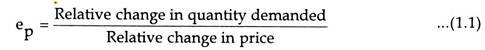
Also, elasticity is the percentage change in quantity demanded divided by the percentage in price.
ADVERTISEMENTS:
Symbolically, we may rewrite the formula:
![]()
If percentages are known, the numerical value of elasticity can be calculated. The coefficient of elasticity of demand is a pure number i.e. it stands by itself, being independent of units of measurement. The coefficient of price elasticity of demand can be calculated with the help of the following formula.
![]()
Where,
Q is quantity, P is price, ΔQ/Q relative change in the quantity demanded and ΔP/P Relative change in price.
It should be noted that a minus sign (-) is generally inserted in the formula before the fraction with a view to making the coefficient of elasticity a non-negative value.
The price elasticity can be measured between two finite points on a demand curve (called arc elasticity) or on a point (called point elasticity).
ADVERTISEMENTS:
Arc Elasticity:
Any two points on a demand curve make an arc. In the words of Baumol, “Arc elasticity is a measure of the average responsiveness to price changes exhibited by a demand curve over some finite stretch of the curve”. The measure of elasticity of demand between any two finite points on a demand curve is known as arc elasticity.
The elasticity coefficient can be calculated with the help of the following formula:
![]()
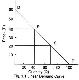
For example, in Fig. 1.1 two finite points R and S are taken to measure the arc elasticity. First we move to measure elasticity for a fall in the price of the commodity from Rs. 40 to 20. ΔP is 40 – 20 = 20. This decrease in price causes an increase in demand from 40 units to 70 so that ΔQ is 40 – 70 = – 30.
These values can be put in the formula so that:
![]()
This implies that a one percent fall in price of commodity X causes a 1.5 per cent increase in demand for it.
ADVERTISEMENTS:
In the measurement, interpretation and use of arc elasticity, the business executives need take adequate care as the elasticity coefficient may differ depending upon the direction of movement. In this case we have measured the elasticity coefficient while moving down from point R to S.
The coefficient will be different while moving upward from point S to R (increase in price from Rs. 20 to 40 and quantity demanded is reduced from 70 to 40 units giving an elasticity coefficient of – 0.42 implying that one per cent increase in price will reduce the quantity by 0.42 percent. Thus the elasticity depends on the direction of change in price. Therefore, measuring elasticity through arc method, the direction of price change should be kept in mind.
The way out of this difficulty is to take an average of prices and quantities and thus to measure elasticity at the midpoint of the arc.
The formula then becomes:
ADVERTISEMENTS:
![]()
Although the ½ cancels out in the formula, it is put there to stress the fact that by using the average values of the quantities and prices, the elasticity coefficient is the same whether price goes up or goes down.
Point Elasticity on a Linear Demand Curve:
Point elasticity is the ratio of an infinitesimally small relative change in quantity to an infinitesimally small change in price. If a price range is made as small as possible, that is, shrunk to a point- then the relative changes must be made as small as possible- infinitesimally small.
ADVERTISEMENTS:
Point elasticity is the ratio of an infinitesimally small relative change in quantity to an infinitesimally small change in price. Point elasticity of demand is defined as the -proportionate change in the quantity demanded resulting from a very small proportionate change in price. Fig. 1.2 shows how to find the elasticity at a point on a demand curve.
Let us take a point such as R on the demand curve DD. For measuring elasticity at a point the following formula may be used.
![]()
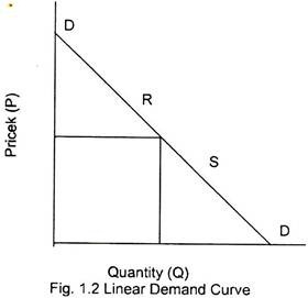
Point elasticity is the product of price-quantity ratio (P/Q) at a particular point (R) on the demand curve (DD) and the reciprocal of the slope of the demand line. The slope of the demand slope is defined by RQ/QD. The reciprocal of the slope of the demand line is QD/RQ.
![]()
ADVERTISEMENTS:
At point R, price P = RQ and Q = OQ
If we substitute these values in equation 1.8, what we get is
![]()
If the numerical values for QD and OQ are available, elasticity at point R can be calculated.
Price Elasticity at Different Points on a Non-Linear Demand Curve:
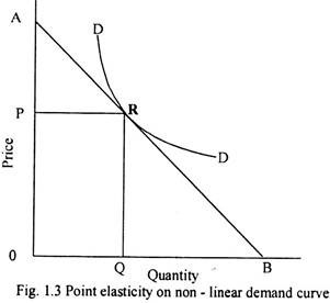
The method used to measure point elasticity on a linear demand curve cannot be applied straightway to measure point elasticity on a non-linear demand curve. In order to measure point elasticity on a non-linear demand curve, we first draw a tangent to the selected point and bring it on a linear demand curve. Fig. 1.3 illustrates how we can measure point elasticity on a non-linear demand curve at point R.
ADVERTISEMENTS:
For this purpose, we draw a tangent AB through point R. Since demand curve DD and the line AB pass through the same point R, the slope of the demand curve and that of the tangent is the same. Therefore, the elasticity of demand curve at point R will be the same as the elasticity on point R on line AB. The formula applied to measure the elasticity on a linear demand curve can now be used as the non-linear demand curve has been changed into a linear demand curve.
Price Elasticity and Total Revenue:
One important application of elasticity is to clarify whether a price increase will raise or lower total revenue. Many business executives are concerned with the issue whether it is worthwhile to raise prices and whether the higher prices make up for lower demand.
Total revenue is equal to price times quantity (TR = P.Q).
If we know the price elasticity of demand, we may know what will happen to total revenue when price changes:
ADVERTISEMENTS:
(1) If price elasticity (ep > 1), reducing the price will increase the total revenue.
(2) When demand is perfectly inelastic ep = 0, there is no decrease in quantity demanded when price is raised. Therefore, a rise in price increases the total revenue and vice versa.
(3) In case of an inelastic demand (ep < 1), the total revenue falls when the price is decreased. The total revenue increases when the price is increased.
(4) When the demand for a product is unitary elastic (ep = 1) quantity demanded increases or decreases in the proportion of increases or decrease in the price. Hence total revenue remains unaffected.
To make this point more clear, we require total and marginal revenue function and price-elasticity of demand.

The MR is then
ADVERTISEMENTS:
MR = Δ(TR)/ΔQ = a0 – 2a1Q … (1.15)
It can be seen from the figure 1.4 that if the demand curve is falling the TR curve initially increases, reaches a maximum, and then starts declining. The derived relationship between MR, P and e can be used to establish the shape of the total- revenue curve.
The total revenue curve reaches its maximum level at the point where ep = 1, because at this point its slope, the marginal revenue, is equal to zero.
MR = P (1 – 1/1) = 0
If ep >1 the total revenue curve has a positive slope. It is still increasing and has not reached its maximum point. If ep <1 the total-revenue has a negative slope and is falling.
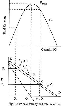
The following can be summarized:
1. If the ep < 1, the demand is inelastic, an increase in price leads to an increase in total revenue, and a decrease in price leads to a fall in total revenue.
2. If ep > 1, the demand is elastic, and increase in price will cause a decrease in the total revenue and a decrease in price will lead to an increase in the total revenue.
3. If ep = 1, the demand is unitary elastic, total revenue is not affected by changes in price because MR has reached zero.
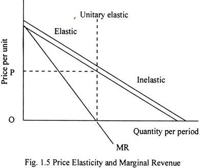
Price Elasticity and Marginal Revenue:
Demand and marginal revenue curves show where demand is elastic, unitary elastic and inelastic. It is clear that demand becomes less elastic at lower prices. This is a characteristic of linear demand curves because the curve is linear dQ/dP is a constant. Thus price elasticity is determined by the value of P/Q. But as price decreases, P/Q also decreases.
Consequently, the absolute value of e becomes smaller and demand becomes less elastic.
The figure 1.5 illustrates that the point of unitary elasticity corresponds to the point where the marginal revenue crosses the quantity axis. The marginal revenue is zero where demand is unitary elastic. Unitary elasticity means that a 1 percent increase in price causes quantity demanded to decrease by 1 percent and the increase in price is exactly offset by the decrease in quantity demanded. Consequently, there is no change in total revenue as the marginal revenue is zero.
The marginal revenue is positive where demand is elastic and negative when demand is inelastic. Note that these relationships are also true for nonlinear demand curves. The point where marginal revenue is zero always divides the elastic and inelastic regions of the demand curve.
In case of a vertical demand curve, quantity demanded is not affected by changes in price as dQ/dP is zero and price-elasticity is also zero. For a horizontal demand curve, quantity demanded is highly responsive to changes in price as even a very small change in price can lead to an infinitely large change in quantity demanded as dQ/dP and price elasticity being infinite. Horizontal demand curves are said to be infinitely elastic. The cases of infinitely elastic or completely inelastic demand curves are rare to find in real life, but an understanding of these is useful for economic analysis.
Method # 2. Income Elasticity of Demand:
The responsiveness of quantity demanded to changes in income is called income elasticity of demand. With income elasticity, consumer incomes vary while tastes, the commodity’s own price, and the other prices are held constant.
The income elasticity of demand for a good or service may be calculated by the formula:
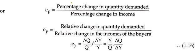
where- ey stands for the coefficient of income elasticity, Y for income.
Whereas price-elasticity of demand is always negative, income-elasticity of demand is always positive (except for inferior goods) as the relationship between income and quantity demanded of a product is positive. For inferior goods the income elasticity of demand is negative because as income increases, consumers switch over to the consumption of superior substitutes.
The degree of income elasticity varies in accordance with the nature of commodities:
1. In case of all normal goods, the income elasticity is positive
2. For essential goods, the income elasticity is less than one. This means that quantity demanded increases less than proportionately as income increases. Soap, salt, match, newspapers have low income- elasticity of demand.
3. For goods of comfort, the income-elasticity coefficient is equal to unit which results in proportionate change in quantity demand.
4. Luxury goods have income elasticity greater than unity implying more than proportionate change in quantity demanded. Jewelry, automobiles are goods of this category.
Income elasticity of demand can be useful in the following business decisions:
1. Income-elasticity can be helpful in production planning and management in the long run, particularly during the period of business cycle.
2. It can be used for demand forecasting with given rate of increase in income.
Income Sensitivity:
The income elasticity of demand measures the degree of responsiveness of physical quantities of consumption of a good as income changes. If we measure consumption by consumer expenditures rather than by physical quantities of a good, the phenomena may be described as income sensitivity. An income- sensitivity may be defined as the percentage change in expenditures on a good divided by the percentage change in income of the consumers.
The income sensitivity may be measured with the help of following formula:
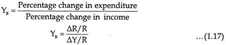
where: Ys measures the income sensitivity, ΔR measures change in consumer expenditure and ΔY measures change in income.
Suppose a 10 percent increase in income causes consumer expenditure on a good to increase by 12 percent, the income sensitivity of that good is 1.2.
Method # 3. Cross Elasticity of Demand:
Demand is also influenced by prices of other goods and services. The cross elasticity measures the responsiveness of quantity demanded to changes in price of other goods and services. Cross elasticity of demand is defined as the percentage change in quantity demanded of one good caused by a 1 percentage change in the price of some other good.
![]()
Cross elasticity is used to classify the relationship between goods. If cross elasticity is greater than zero, an increase in the price of y causes an increase in the quantity demanded of x, and the two products are said to be substitutes. When the cross- elasticity is greater than zero, the goods or services involved are classified as complements Increases in the price of y reduces the quantity demanded of that product. Diminished demand for y causes a reduced demand for x. Bread and butter, cars and tires, and computers and computer programs are examples of pairs of goods that are complements.
The coefficient is positive if A and B are substitutes because the price change and the quantity change are in the same direction. The coefficient is negative if A and B are complements, because changes in the price of one commodity cause opposite changes in the quantity demanded of the other. Other things such as consumer taste for both commodities, consumer incomes and the price of the other commodity are held constant.
Many companies produce several related products. Where a company’s products are related, the pricing of one good can influence the demand for other products. Gillette makes both razors and razor blades. Ford sells several competing makes of automobiles. Gillette probably will sell more razor blades if it lowers the price of its razors.
The closer two commodities are as substitutes for each other, the greater is the size of the cross elasticity coefficient. Close substitutes have high cross elasticity of demand; poor substitutes have low cross elasticity.
In general, a rise in the price of a commodity increases the demand for its substitutes and diminishes the demand for its complements.
Method # 4. Advertisement or Promotional Elasticity of Sales:
The advertisement expenditure helps in promoting sales. The impact of advertisement on sales is not uniform at all level of total sales. The concept of advertising elasticity is significant in determining the optimum level of advertisement outlay particularly in view of competitive advertising by rival firms. An advertising elasticity could be defined as the percentage change in quantity demanded for a percentage change in advertising. Advertising might be measured by expenditure.
Advertising elasticity may be measured by the following formula:
![]()
where: S = sales; ΔS= increase in sales; A = initial advertisement outlay; and ΔA = increased advertising outlay.
The advertising elasticity of sales varies between zero and infinity. If advertising elasticity is zero, sales do not respond to the advertising expenditure. Promotional elasticity coefficient greater than zero but less than 1 (eA>0<1) indicates that sales increase less than proportionate to the increase in advertisement expenditure. The coefficient of equal to 1 means proportionate increase in sales to the increase in expenditure on advertisement. If eA > 1 it interprets that sales increase at a higher rate than the rate of increase of advertisement expenditure.
Determinants of Advertisement Elasticity:
1. The Level of Sales:
The advertising elasticity of sales, particularly in case of products newly introduced into the market, is greater than unity. Sales increase more than proportionately with the increase in advertisement expenditure. As sales increase elasticity begins to decrease. Now the advertisement is done to create new customers to the product. Therefore, demand now increases less than proportionately to increase in advertisement.
2. Competitive Advertising:
The advertising elasticity of a firm will depend not only on the advertisement expenditure incurred by the firm for its product but also on the effectiveness of the competitive advertising by the rival firms
3. Cumulative Effect of Past Advertisement:
In the initial stages the advertisement outlay is not adequate enough to be effective. Therefore, the elasticity may be very low. But in later stages as the cumulative effect of advertisement gather, the advertising elasticity may increase over time.
Change in product’s price, consumer’s income, increase in the number of substitutes and their prices are other factors that influence the advertising elasticity of a product.
Method # 5. Elasticity of Price Expectations:
People’s price expectations also play a significant role as a determinant of demand. J.R. Hicks, the English economist, in 1939, devised the concept of elasticity of price expectations. The elasticity of price expectations may be defined as the ratio of the relative change in expected future prices to the relative change in current prices.
![]()
![]()
where,
Pc Current prices
Pf Future prices
If ex > 1 Buyers expect that future prices will rise by a larger percentage than current prices.
ex = 1 Buyers expect that future prices will rise by the same percentage as current prices.
ex < 1 Buyers expect that future prices will rise by a smaller percentage than current prices.
ex = 0 Buyers expect current rise to have no effect on future prices
ex < 0 Buyers expect that current rise will be followed by a fall in future prices.
The concept of elasticity of price-expectation is very useful in formulating pricing policy.