Externalities in Production and Consumption

In this article we will discuss about the externalities in production and consumption.

Introduction to Externalities:

The conditions for efficiency in consumption and production and overall economic efficiency. These conditions involve marginal rates of substitution (MRS) and marginal rates of product transformation (MRPT). The conditions were derived on the assumption that there were no external effects in consumption and production.

However, this may not be so always. Consumption and production may be subject to externalities. The externalities could be positive (these involve external benefits) or negative (these involve external costs).

We may first give some examples of positive and negative externalities and then discuss how they change the marginal conditions of efficiency:

(i) Positive Externality in Consumption:

An example of this is vaccination. The welfare of any person in a particular neighbourhood depends not only on whether he is vaccinated but also on whether the people in the said neighbourhood have been vaccinated so that the contagious diseases are not spread.

(ii) Negative Externality in Consumption:

The welfare of any person in a particular neighbourhood depends not only on his avoidance of riding a noisy motor cycle, but also on other people’s avoidance of doing this.

(iii) Positive Externality in Production:

The example which is often cited here is that of the production of honey. Beekeepers try to put their beehives on farms because nectar from the plants increases the production of honey. The farmers also receive advantages from the beehives because the bees help pollination of the plants.

(iv) Negative Externality in Production:

A very suitable example is that of a paper mill that produces paper and the waste is dumped into a river. The riverside residents and the fishes are hurt by the waste.

Consequences of Externalities:

We may now analyse the consequences of these externalities. The British economist A. C. Pigou was the first to deal with externalities in a systematic way. Pigou argued that in the presence of externalities we do not achieve a Pareto optimum even under perfect competition. If the externalities are present, the social benefit or cost resulting from the production of goods becomes a combination of private and external benefits or costs.

Let us use the following notations:

MPC = marginal private cost

MEC = marginal external cost

MSC = marginal social cost and, by definition,

MSC = MPC + MEC Also,

MPB = marginal private benefit

MEB = marginal external benefit

MSB = marginal social benefit and, by definition,

MSB = MPB + MEB

Now, overall economic efficiency requires MSC = MSB for each product. For, as long as MSB > MSC, production should be expanded, because additional benefit exceeds additional cost; on the other hand, if MSB < MSC, then production should be decreased in order to avoid the marginal inefficiencies.

Consequently, we should have, for each pair of products, equality between the marginal social rate of product transformation (MSRPT) and the marginal social rate of substitution (MSRS) between the goods. In the presence of externalities, if only the marginal private costs are considered, the economy will not reach economic efficiency.

That is, for economic efficiency, consumers and producers must weigh the full social benefits and costs of consumption and production. One way to achieve this is to impose taxes and subsidies which bring private benefits or costs into line with social benefits or costs. We will now illustrate how these taxes and subsidies would work.

Negative Externality in Production:

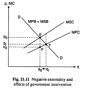
The case of a negative externality in production has been illustrated with the help of Fig. 21.11. Here we are assuming that there are no externalities in consumption. That is why the demand curve DD shows the marginal private and social benefits (MPB = MSB).

On the other hand, owing to the presence of externalities in production, the marginal social cost (MSC) curve is different from the marginal private cost (MPC) curve, the latter representing the competitive supply curve.

In the case of a negative externality, MSC would be greater than MPC, i.e., the MSC curve would lie above the MPC curve as has been shown in Fig. 21.11. The optimal output here is q₀ with the price p₀. But the competitive market, if left alone, will produce q₁ at the price p₁. Thus, there would be a tendency to overproduce in the absence of any market intervention.

At the optimal quantity q₀, the price would be p₀, but the MPC would be c₀. Thus, the government could levy a per unit tax of (p₀ – c₀) on the firm, and thereby increase the MPC by (p₀ – c₀), i.e., to the level of MSC. Consequently, the output of the firm would diminish to q₀ (from q₁). The consumers would pay the price p₀ = MSC.

Now, the revenue from the tax could be used to pay for the external damage caused by the production of the commodity. Let us note, however, that the tax revenue could be more or less than the external damage.

The revenue would be equal to (p₀ – c₀) x q₀ = □p₀EFc₀ whereas the total external cost would be equal to the area between MSC and MPC curves up to q = q₀. Finally, the net gain to society from the tax is given by □EFT which is the excess of MSC over MPC over the range of output from q₀ to q₁.

Positive Externality in Production:

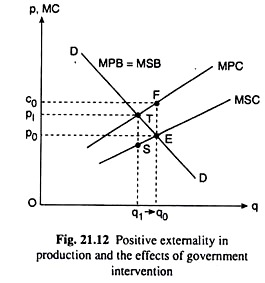
This case has been illustrated in Fig. 21.12. In this case, since there are external benefits, the MSC would be less than MPC and the MSC curve would lie below the MPC curve. In the absence of any externality in consumption, the demand curve for the good gives us the marginal social and private benefits (MSB = MPB).

Therefore, the optimal output would be given by the point of intersection E between the demand curve DD and the MSC curve.

This optimal output is q₀ at the price p₀. At this output, we have MSB = MSC. However, if there is no market intervention, the competitive market will produce q = q₁ at the point of intersection T between the demand curve DD and the competitive supply curve MPC.

In this case of external benefits in production, the free market will produce less than the optimal output (q₁ < q₀). At the optimal level of output, the producers will receive a price p = p₀, but their marginal cost is MPC = c₀.

Since c₀ is greater than p₀, the producers would have to be paid a subsidy of (c₀ – p₀) if they are to increase the output level from q₁ to the optimal level q₀. In the earlier case of external cost a per-unit tax equal to the marginal external cost needed to be imposed to arrive at the optimal output level.

On the other hand, in the present case of external benefit, a per-unit subsidy equal to the marginal external benefit has to be given to the producers.

Now, the government may collect the money to be paid as subsidy from the people enjoying the external benefit. But here again, the expenditure on the subsidy [- (c₀ – p₀) x q₀ = □P₀EFC₀] may not be equal to total external benefit [= the area between the MPC and MSC curves up to q = q₀].

Finally, the net benefit to society from the subsidy would be equal to □STE which is the excess of social benefit over social cost over the range of output from q₁ to q₀.

Negative Externality in Consumption:

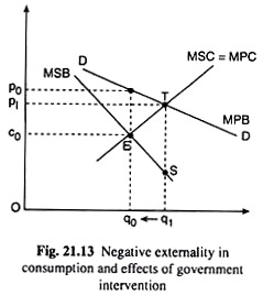
This case has been illustrated in Fig. 21.13. Since there are no externalities in production, MSC and MPC curves are identical .and either of them represents the competitive supply curve. However, on the demand side, the demand curve DD reflects only the marginal private benefit (MPB).

In the presence of negative externality in consumption, the marginal social benefit (MSB) is less than the MPB. That is why the MSB curve lies below the MPB or the DD curve. The socially optimal quantity again is q₀ at the MSC = MSB point, E, and the price is p₀.

However, in the absence of any intervention, the quantity supplied and demanded is q₁ at the point of intersection T of the DD (or MPB) curve and the MPC = MSC curve, and the price here is p₁. Thus, there is an overproduction of the commodity (q₁ > q₀) as compared to the socially optimal level.

If the output is to be restricted to the optimal level, q₀, the price has to be raised to p₀. But the supply price at q = q₀ is c₀. Hence, a tax equal to (p₀ – c₀) per unit needs to be levied. Then the consumer would pay the price p₀ including the tax which is equal to MPB, i.e., c₀, plus the cost of externality in consumption which is (p₀ – c₀).

Here the revenue generated from the tax may be used to compensate those who are harmed by the negative externality of the consumption of the product. Also, the area EST represents the net benefit of the tax to society. This area is equal to the excess of MSC over MSB over the range of output from q₁ to q₀.

Positive Externality in Consumption:

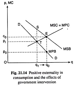
This case is illustrated by means of Fig. 21.14. In the absence of externality in production, the MSC and MPC curves are identical and either of them represents the competitive supply curve. But on the demand side, the demand curve DD represents only MPB. In the case of positive externality in consumption, we have MSB > MPB, i.e., the MSB curve would lie above the DD curve or the MPB curve.

Given all this, the socially optimal level of output in Fig. 21.14 is obtained to be q₀ at the MSB = MSC point E, the price of the output being p₀. Without any intervention, the quantity produced would be q, at the MPB = MPC (= MSC here) point T.

Since q₁ < q₀, there would be underproduction of output (as compared to the socially optimal level) in this case of positive externality in consumption. At q = q₀, the market price would be p₀ but the marginal cost (both private and social) would be c₀. Since the marginal cost (c₀) is greater than the price (p₀), the producers have to be given a per unit subsidy of (c₀ – p₀) if the output is to be maintained at the optimal level, q₀.

Then the producers will get c₀ per unit of output and the consumers would pay p₀. At least part of the subsidy (c₀ – p₀) x q₀ could possibly be collected from those who reaped the external benefits arising from the consumption of the good. Again, the net benefit to the society from the subsidy is measured by the area EST which is the excess of social benefit over the social cost over the range of output from q₁ to q₀.

Summary:

In the cases of externalities discussed above we have obtained the following results:

(i) In the presence of externalities, the socially optimal level of output q₀ is given by the condition MSB = MSC.

(ii) The private production of output q₁ is given by the condition MPB = MPC.

(iii) To obtain the optimal level of output q₀, we can use some appropriate tax and/or subsidy programmes.