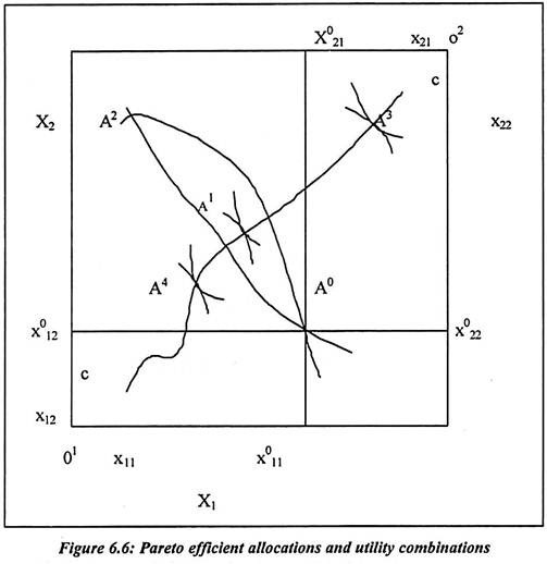
Edgeworth diagram is divided into two types. The horizontal side of the box measures a fixed total output of good 1 and the vertical side measures a fixed total output of good 2. Individual 1’s consumption of good 1 is measured horizontally from the origin at o1. His/ her consumption of good 2 is vertical from o1. In the diagram, consumption of individual 2 is measured from the origin at o2. The Edgeworth box diagram assumed that there is non-satiation of consuming commodities.
It means that it cannot be efficient to have total consumption of any good which is less than the output of the good. Therefore we need to restrict attention to consumption bundles for the individuals. It will add up to the total output of the two goods. In the Edgeworth box diagram, a single point is defined as the consumption bundle of both individuals. The allocation A0 has individual 1’s allocation and he is getting the consumption bundle (x011, x012).
The individual 2 is getting (x021, x022) the consumption bundle. If we assume that the individual labour supply is constant then we need to draw different indifference curve. We can draw another indifference curve for two commodities. Such indifference curves are drawn for two commodities. Both the individuals have strictly quasi-concave utility function. Therefore the indifference curves for individuals are convex to their origin.
In the Edgeworth box diagram, the allocation A0 is not Pareto efficient. It is possible to exchange commodities between two individuals so as to make them both better off. The allocation A’ is Pareto superior than A0. Such new allocation puts both individuals on indifference curves. It is further from their respective origins. The A2 allocation in the diagram is inversely of the A0 allocation. It is lens shaped area and it is defined by the indifference curves through A0.
ADVERTISEMENTS:
The allocation A2 is superior to A0. In the above diagram, allocation cannot cross the indifference curves. This is because all allocations are Pareto efficient. There are different allocations in the box diagram. The indifference curves are tangent at A1, A3 or A4. All tangent point in the box diagram is efficient. The indifference curves and its slope are negative. It is because of the marginal rate of substitution.
In the box diagram, the locus cc of points of tangency between the indifference curves. Such point is a tangency between two curves. Such points are set of all Pareto efficient allocations of given total output. It is measured both sides of the diagram. In the exchange economy that is barter system where goods are exchanged for goods, the consumers have fixed endowments of consumption goods. The efficient consumption conditions are required for the Pareto efficiency.
In the box diagram, each allocation and point generates the utility combinations. Such utility combinations are written as (u1, u2). The Pareto efficient allocations on the curve cc would generate utility combinations. Such utility combinations of the individuals are considered as utility frontiers. The inefficient allocations would generate combinations inside the utility frontier.
ADVERTISEMENTS:
Efficient Input Supply:
For the efficient input supply, we need to combine the equation 55, 56, 57, and 58.
Such equations yield the further equation as follows:
From equation 59 and equation 60, we can derive another function. It is as follows:
From the above equation, we need to consider the efficiency and its further implication. They are presented as follows:
The MRS in the above equation means h’s marginal rate of substitution. It is between input supply and consumption of commodity i. It is further defined as the rate at which h must be compensated by being given more of commodity i. It is possible when consumer increases supply of Zh by one unit. The right hand side of equation 63 is the marginal product of Zh in the production of commodity i.
The Pareto efficiency requires that the additional output produced by an extra unit of Zh is just equal to the marginal cost. It is in terms of good i of Zh to h. Suppose we assume that h can be compensated by two units of good i for supplying one unit of Zh then it can be used to increase output of good i by 3 units. Such allocation cannot be Pareto efficient and it is true for the above case.
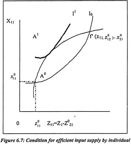
We have also derived the figure which shows the condition for efficient input supply. Such efficient input supply is given by individual 1. All the consumption level except and all input uses except z11, are held constant. In the diagram, the vertical axis plots the consumption of good 1 by individual 1. It is denoted as x11 = x1 ⎯ x021. The horizontal axis plots the use of his input by firm 1. It is denoted as z11 = z1 ⎯ z021. With all other consumption and input use fixed increases in z1 imply equal increases in z1. Thus we can show the indifference curves of individual 1 in (z11, x11) space as Io, I1.
In the diagram, these curves are just the counters of u’ (x11, x012 z1) = u'(x1, x021, x021z11 + z021). The curve f’-plots f’ (z11, z012)-x021 against z11. It shows the effect of variations in z11 on the consumption of good 1 by individual 1.
Suppose the initial allocation is A0 then the consumption of good 1 by individual 1 is x011. The use of input by firm 1 is z011. At allocation A0, the indifference curve I0 cuts the curve f’-x021. This is because by shifting allocation A’, individual 1 achieve a higher utility level of I’. It is only when the indifference curves of individual 1 are tangent to the curve f’- x021. Such effect is considered as the efficient allocation.
ADVERTISEMENTS:
The slope of the curve is given by equation as f’-x021, is ∂[f’’(z11, z012) ⎯ x021]/∂z11 = f11. The marginal product of input 1 is the production of good 1 and the slope of the indifference curve is (x11, z1 ⎯ z021). The space is just individual 1’s marginal rate of substitution between commodity 1 and his input supply. Therefore we have again established the efficient input supply condition. The equation 63 is necessary for efficiency condition.
Efficient Input Use:
From the equation 59, we can use a given total supply of inputs by the firms. It gives us the following equation which we have defied as,
ADVERTISEMENTS:
The ratio of the marginal products is f11/f12. It is the marginal rate of technical substitution. The MRTS121 of input 1 for input 2 is the production of good i. The MRTS121 is the rate at which input 1 can be substituted for input 2 without change in the output of good i.
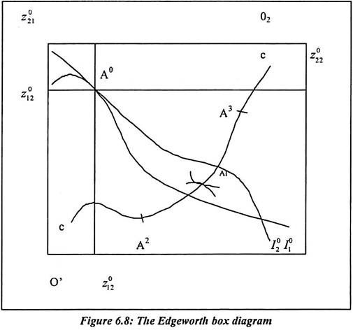
In the following figure 5.8, the feasible allocation increase in z11 by one unit reduces z21 by one unit. Further it reduces z12 by four units and it increase z22 by four units. The net effect will be to increase the output of both goods. The initial allocation cannot have Pareto efficient. The equality of marginal rate of technical substitution for firm is necessary for efficiency. The following diagram shows the Edgeworth box diagram. It shows the fixed input supplies of the two individuals. It is measured by the lengths of the sides of the box.
Firm 1 uses of the input which is measured from the origin 02, but it cannot be efficient for the total use of an input to be less than the supply. Now we can restrict attention to allocations. But the allocation is Σi zih = zh.
ADVERTISEMENTS:
In the Edgeworth box diagram, the allocations are defined by a point A0. Here, we assume that the production function is strictly quasi-concave. The iso-quant for firm 1 is the curve like I01 and for firms 2 the curve is I02. We have assumed that marginal products are positive. They are intersecting each other at larger output. The allocation A0, is the iso-quant where two firms have cross curve where the points are not efficient.
They always exists other feasible allocations like A’. Such point produces more of the both output. At A’ point, the iso-quants are tangent and they are the efficient points. The slope of iso-quants is the firm’s marginal rate of technical substitution. Such MRTS yields the equation 64. It is necessary condition for efficient use of a given supply of inputs.


