Combining Goods Market and Money Market (With Diagram)

Goods market and money market do not op­erate independently—one influences the other.

Thus, combining these two markets, we determine the values of Y and r that are con­sistent with equilibrium in these two markets.

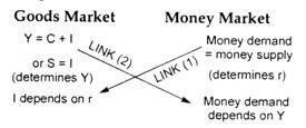
The interrelationships or the links between these two markets are:

There is a link between investment and interest rate determined in both the goods market and money market.

Investment is as­sumed to be determined by interest rate in a negative fashion. We have amply demon­strated here that the interest rate has been determined in the money market. Thus, money market influences goods market.

Another link can be traced between out­put/income and demand for money. We have seen that aggregate output determined in the goods market influences demand for money. An increase in income (keeping interest rate constant) causes an increase in money de­mand.

These two links can be shown in the fol­lowing form:

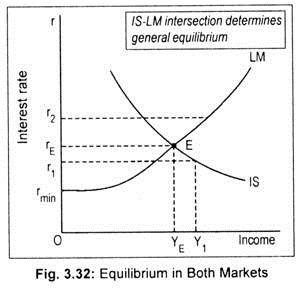
Fig. 3.32 shows the general equilibrium in terms of IS and LM curves. Here, when both the curves are plotted on the same axes, the equilibrium level of income, Y_E, and the equi­librium interest rate, r_E, are determined si­multaneously. This is known as the synthesis of monetary analysis and income analysis or macroeconomic general equilibrium. Point E is the (only) point of general equilibrium for both the markets. Point E is a stable equilib­rium point.

To demonstrate stability, let us consider r₁ – Y₁ combination. Since this combination is on the IS curve, the product market is in equilibrium while money market is not. At this combination, there is an excess demand for money (EDM). To meet this excess demand, people will go on selling bonds. This will de­press bond prices and raise interest. As inter­est rate increases, there are repercussions in the product market.

Now, following an in­crease in interest rate, investment declines and, as a consequence, income declines. So, interest rate and national income will go on changing until point E is reached, if the equi­librium is to be a stable one. This occurs only at r_E and Y_E.

Similarly, any r – Y combination above r_E (say, Or₂) will exhibit equilibrium in the money market, but disequilibrium in the product market. Now, product market will experience a deficiency in aggregate demand.

This causes income to decline. As income declines, there are repercussions in the money market. Now, demand for money will decline as income declines. So, rate of interest must decline. If the equilibrium is stable, r and Y tend to change until point E is reached. Thus, E is a stable equilibrium point. One thing should be borne in mind—to have stability in equilibrium, the slope of the IS curve must be less than that of the LM curve.

A Mathematical Example on General Equilibrium:

Given C = Rs. 150 + 0.50Y, I = Rs. 200 – 400r, M_d = 0.25Y, M_s = Rs. 50 – 100r and M = Rs. 180. From these information, we like to determine equilibrium level of income, consumption, investment, transaction and speculative demand for money.

Step 1:

Product market equilibrium needs to be determined.

Equilibrium condition for the product market is:

Y = C + I

.^.. Y = (Rs. 150 + 0.50Y) + (Rs. 200 – 400r)

(Y- 0.50Y) = 150 + 200 – 400r

or 0.50Y = 350 – 400r (IS equation)

Step 2:

Money market equilibrium requires money demand must equal money supply.

M = M_d + M_s

.^.. Rs. 180 = 0.25Y + 50 – 100r

or 0.25Y = 130 + 100r

or 0.50Y = 260 + 200r (LM equation)

Step 3:

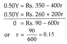
Combining equilibrium goods market and money market equations, we obtain

Step 4:

Putting the value of r in either IS or LM equation we get the value of Y:

Y = Rs. 580

Step 5:

C = Rs. 440

Step 6:

I = Rs. 140

Step 7:

M_d = Rs. 145

Step 8:

M_s = Rs. 35