Factor Productivity and Factor Cost | Theories of Distribution

The below mentioned article provides an overview on the concepts of factor productivity and factor cost.

Concepts of Factor Productivity:

There are two main concepts relating to factor productivity: physical productivity and revenue productivity,

(i) Physical Productivity:

When we express the productively of any factor in terms of goods and services, it is called physical productivity. It is further divided into average and marginal physical productivity.

(a) Average Physical Productivity (APP). APP is the physical units produced per unit of the variable factor. It is arrived at by dividing total physical productivity (TPP) by the number of units of the variable factor employed (N), i.e.

APP = TPP/N

(b) Marginal Physical Productivity (MPP). MPP is the addition made to total output by employing an additional unit of a variable factor.

MPP = TPP – TPP_n-1,

(c) Value of Marginal Physical Productivity (VMPP). The value of marginal physical productivity (or product) is obtained by multiplying MPP with the price (AR) of the product

VMPP or VMP = MPP x Price (AR)

(ii) Revenue Productivity:

When we express the productivity of a factor in terms of money, it is called revenue productivity. It is further divided into average and marginal revenue productivity.

(a) Average Revenue Productivity (ARP):

ARP is the revenue obtained per unit of the factor employed. It is obtained by dividing total revenue productivity (TRP) by the total number of units of the factor employed (N) i.e.

ARP = TRP/N

It is also obtained by multiplying APP with the price of the product.

ARP = APP x Price (AR)

(b) Marginal Revenue Productivity (MRP):

MRP is the addition made to total revenue productivity by employing one more unit of a variable factor, i.e.,

MRP = TRP_n – TRP_n-1

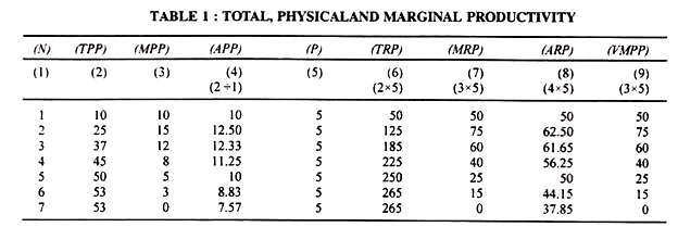
The relation between physical, marginal and average productivity under perfect competition is shown in Table 1.

Relation between ARP and MRP:

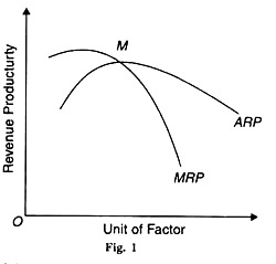
There is a definite relation between ARP and MRP curves which is based on the Law of Variable Proportions. Both ARP and MRP curves are inverted (u-shaped or bell (ᴖ) shaped. First they rise upward, reach a maximum and then decline, as shown in Figure 1.

The relation between the two is as follows:

(1) When the ARP curve rises, the MRP curve is above it.

(2) When the ARP curve is at its maximum, a point M, the MRP curve cuts it from above.

(3) When the ARP curve falls, the MRP curve is below it and falls steeply.

Concepts of Factor Cost:

The total cost of a factor (TFC) is the expenditure incurred by a firm in hiring or buying that factor. It is further divided into average and marginal factor cost.

(a) Average Factor Cost (AFC). AFC is the per-unit cost of the variable factor employed by a firm. It is obtained by dividing total factor cost by the units of the factor employed, i.e..

AFC = TFC/Units of Factor Employed

(b) Marginal Factor Cost (MFC). It is the addition to the total factor cost by hiring or purchasing an extra unit of that factor:

MFC = TFC_n – TFC_n-1

Table 2 expects the costs concepts and their relation under perfect completion:

Relation between AFC and MFC:

The relation between AFC and MFC is different in a perfectly competitive factor Market and monopolistic factor market. In a perfectly competitive factor market, the price of a factor is determined by its demand and supply.

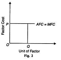
The price of that factor is given for the firm at which it buys as many units as are required by it. Therefore, the supply of the factor is perfectly elastic at the given price and the supply curve of the factor is a straight line paralleled to the x-axis.

As the price of the factor is assumed to be given and constant, therefore its average factor cost and marginal factor cost equal the price of the factor i.e., AFC = MFC = Price of the Factor. This relationship is shown in column (2), (4) and (5) of Table 2 and in Figure 2 where the supply curve of the factor is P = AFC = MFC at which its OQ quantity is bought by the firm.

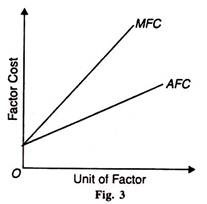
In a monopolistic (imperfect) factor market, a firm had monopsony, being the sole buyer of a factor.

So its factor supply curve (AFC) is upward sloping to the right and its MFC curve is above its AFC curve, as shown in Figure 3. It means that if the firm wants to employ more units of that factor (say labour), it will have to spend more (wage) not only on additional units but on its all units (workers). Consequently, MFC of that factor will be more than its AFC (actual cost). Therefore, the MFC curve will be above its AFC curve.