
The theory of distribution deals essentially with the determination of the levels of payment to the various factors of production, i.e., the prices of the economy’s productive resources. The theory of income distribution is related to factor pricing. It is a segment of general equilibrium theory, inasmuch as a change in the level of wages, interest rates, or rents has significant effects on the whole economy.
As W.J. Baumol has put it- “Since general equilibrium analysis seeks to account for the determination of every price in the economy, it includes the pricing of inputs within its scope.”
Two Sets of Theories:
The theories of distribution can be broadly divided into two categories, viz., microeconomic theories and macroeconomic theories. The most celebrated microeconomic theory is the marginal productivity theory of distribution. It was developed by J.B. Clark in 1899 and then modified by Philip Wicksteed. The two macroeconomic theories are the classical (Ricardian) theory and the Cambridge (Kaldor) theory. Although Karl Marx was very much concerned about the ethical aspects of distribution theory, he never formulated any model (theory) of distribution Marxian economic analysis is related primarily to production.
ADVERTISEMENTS:
1. Marginal Productivity Theory:
The marginal productivity theory is an approach to explaining the rewards received by the various factors of production that jointly produce output. It holds that the wage rate or payment for the services of a unit of a factor is equal to the decrease in the value of commodities produced that would result if any unit of that factor were withdrawn from the productive process, the amounts of all other factors remaining the same.
The basic justification of this assertion is simple enough. It rests on three assumptions: that the products sold are produced by technologies that satisfy the ‘law of variable proportions’ which holds that successive equal increments of one factor of production, the amounts of all other factors remaining unchanged, will yield successively smaller increments of physical output.
It follows immediately from these assumptions that if the wage of any factor exceeds the value of the output that would be lost if a unit less of that factor were employed, then a unit less of that factor will be employed, and successive units will be released until the inequality is annihilated.
ADVERTISEMENTS:
Similarly, if the wage of any factor is less than the value of the output that an additional unit could produce, successive units of that factor will be employed until the inequality disappears. The essence of the marginal productivity (MP) theory is very intuitive: under pure competition the profit-maximising firm will hire any factor (such as labour) up to the point where its price (wage) equals the value of its marginal product, i.e., MPPL x P.
The reason is that if the VMP exceeds the price of the factor, the firm can increase its profits by acquiring additional units of the input since more units bring in more revenue to the firm than they cost. The reverse is true if the price of the factor exceeds its VMP.
For a single product firm, whose production function is q = f(f1, f2,…., fn). where f1 is the quantity its i-th factor, profit is given by:
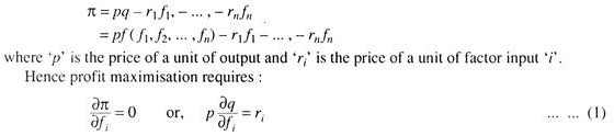
If there is imperfection in the commodity market and price of the product of a firm varies with output, the return to the input will be equated to its MRP (= P x MPP – the loss in revenue of the firm that results due to the fact that increased production forces it to reduce its price of all the previous units).
ADVERTISEMENTS:
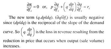
In this case the profit-maximisation requirement becomes:
In Fig. 1 DD is the firm’s demand curve. Suppose an additional unit of input increases output from qa to qb (MPP = qb– qa). Thus, the VMP is equal to the price multiplied by (qb– qa). This is shown by the area CqaqbB. However, price fall leads to a loss on the initial units, shown by the area PaPbCA. The difference between the two shaded areas is the MRP of the output. The firm will hire the input until its price is equal to that MRP.

Evaluation:
At present the marginal productivity principle is used to explain the demand for factors of production in both a two-factor version using aggregate capital and aggregate labour as the factors, and an n-factor version, where n is the number of distinguishable factors used in the production process.
To use the two-factor version it is necessary to establish quantitative measures of the aggregates of dissimilar objects that are given the names ‘capital’ and ‘labour’, a task that has never been performed to anyone’s satisfaction.
According to Milton Friedman and W.J. Baumol, the marginal productivity theory is essentially a theory that helps us to determine the firm’s derived demand for any given input. It shows how the quantity of the input demanded by a profit-maximising firm will vary with the input’s price and makes it abundantly clear that, for such a firm, this demand relationship depends directly on the demand for the final product as well as the input’s marginal physical product (i.e., its extra contribution to total output of the firm).
ADVERTISEMENTS:
In truth, the marginal productivity theory is not a theory of input price determination. It analyses how a firm takes any decision regarding the optimal usage of an input. But it fails to explain how usage and prices of other inputs are determined. The reason is that it ignores the supply side of the input market completely.
Very frequently, if the problem of finding the combination of factor inputs that maximises profits is solved in a straightforward way, some of the input levels in the solution turn out to be negative—which is nonsense. The essential perceptions of marginal productivity theory still apply, but they can no longer be expressed by equalities between price ratios and ratios of marginal changes.
Moreover, the marginal productivity theory has to be cast in general equilibrium framework of the Walrasian type by collecting information on each input (whether purchased from another firm or a private individual like a worker selling his labour power) as also on demand for and supply of every good produced in the economy.
Otherwise it is not possible to find out a set of equilibrium prices and quantities for every item in the economy, including wages for different types of labour (skilled, semi-skilled and unskilled), rents for different qualities of land, etc. If this is done, then only the marginal productivity theory will turn out to be a generalized theory of factor price determination.
ADVERTISEMENTS:
No partial model is adequate for the purpose of building such a theory because a rise in wages in industry ‘A’ will sooner or later raise labour costs in industry ‘B’. A rise in the price of fuels will affect the relative demands of other inputs.
The relevant question here is not whether marginal productivity theory (with necessary modifications) is valid or logically defective. Instead, the issue is the degree to which it is useful. The truth is that the theory, with all its assumptions, is fundamentally valid but perhaps not so illuminating as one might expect.
Theory and Evidence:
The real test of a theory lies in its empirical verification. By using the Cobb-Douglas production function (CDPF) at the aggregate level, economists have attempted to test the empirically observed fact that the share of wages in the national income of the USA has remained relatively constant for a fairly long period of time.
ADVERTISEMENTS:
At the macro-level the CDPF takes the following form:
Y = mLαK1-α
where, ‘m’ and a are positive constants (and α < 1). Here ‘F is national income, ‘L’ is the quantity of labour input and ‘K’ is the quantity of capital employed. If labour is paid a wage equal to its marginal product this production function will yield a share of wage relative to total output which has a fixed value and is independent of the values of the variables Y, L and K, as the empirical evidence suggests. In fact, the ratio between total wage income and total output, K, must, in this case, be exactly equal to a, the exponent of labour (L) in the CDPF. The same result is obtained in case of the income of capital.
Proof:
Here MPL = α mLα-1 K1-α.
Since this is the wage per worker, total wage payments must equal its amount multiplied by the number of workers, L; i.e., the total wage bill must be:
ADVERTISEMENTS:
L αmL(α-1)K (1-α) = α mLαK(1-α) = αY.
Thus, total wage bill equals α times total output.
One question which remains unanswered is why, in spite of rapid technological progress in the USA, the exponent of the production function (α) has not changed. Thus, the explanation of a constant wage share goes in terms of a constant α, for which no explanation is offered.
Critics also comment that there is no valid reason for accepting the basic proposition that the CDPF gives an accurate depiction of technology at the macro-level (i.e., for the economy as a whole). It is just an empirical thesis which has been proposed to explain an empirical observation.
Euler’s Theorem and the Adding-up Controversy:
The second application of the marginal productivity theory was in the area of distributive justice. J.B. Clark believed that distribution of factor incomes according to the marginal product of each factor gives every factor an amount of social output the factor (or the agent production) creates. Thus, the distribution of income on the basis of the marginal productivity theory seems to be equitable in nature.
ADVERTISEMENTS:
For this reason some economists attempted to use the theory as a basis for showing that the distribution of income under free competitive capitalism must be morally just. As a result, it became important to the proponents of the theory to show that the sum of the marginal products added up to exactly the total product, leaving neither a deficit nor a surplus for the entrepreneur to extract.
In this context, the Euler’s theorem comes to our aid. The theorem tells us that if the production functions is linearly homogeneous, i.e., it shows CRS, the sum of the marginal products, will actually add up to the total product.
This means that if each input ‘i’ is paid ri = p ∂q/∂fi, the value of its marginal product, we must have:
![]()
Philip Wicksteed’s injection of linear homogeneous production function into the discussion of distribution theory opened a heated and prolonged controversy over the plausibility of the hypothesis that the production function will really take this form.
According to Samuelson, whether there are any profits of exploitation left over for the capitalist to realise is really a matter of market conditions. Only in monopoly there will be profit in excess of other factor incomes. But, in perfect competition, long-run profit will be zero—since each factor is paid on the basis of its marginal product.
ADVERTISEMENTS:
It was initially proposed by Leon Walras and then rediscovered by J.R. Hicks that whether or not the production function is linearly homogeneous in the vicinity of a competitive equilibrium point it must be locally linearly homogeneous, that is, all of its values and derivatives must be the same as those of a linearly homogeneous function.
Thus, at that point all of the marginal products (the partial derivatives ∂qi/∂fi) must coincide with those of a linearly homogeneous function and so they too must satisfy the Euler’s theorem condition which says that marginal products add up to the total product. In this context, W.J. Baumol has suggested an explanation of why the production function must be locally linearly homogeneous in competitive equilibrium.
It may be noted that the simple function
C = r1f1 + r2f2 + … + rnfn … (2)
must be linearly homogeneous in the input quantities f1 , f2,… ,fn , since if each fi is multiplied by λ then C (total factor cost) will also be multiplied by λ and that is the implication of linear homogeneity. Now equation (2) is the total factor cost of the firm and its graph is the (hyper) plane through the origin, CaCbCcCd, in the two-input case shown in fig. 2. The shaded area (surface) of the diagram represents the production function (or, in this context, the value of output) PI = pf(L, K), in case of two variable factors (labour and capital).
If the second order conditions hold at the point of equilibrium, T, the two surfaces must be tangent there, since the requirement of zero (excess) profit ensures that at no combination of inputs and outputs will the value of output exceed the cost of the corresponding inputs and at the equilibrium point the two will be the same. In fact, the tangency of the two surfaces at T means that they will have the same derivatives.

Alternatively stated, pf (L, K) must, indeed, be linearly homogeneous locally at T. Euler’s theorem must, therefore, apply, and the payment to each factor on the basis of its marginal product must exhaust total product.
Criticisms:
No doubt, the marginal productivity theory is the basis of most theoretical discussions on the issue of distribution. However, with all its restrictive assumptions, most notably those of universal perfect competition and stationary equilibrium, it is not a very accurate representation of reality.
As Baumol has put it:
“What is claimed is that it describes a consistent mechanism which bears at least some resemblance to the workings of our economic institutions and that embodied within its general equilibrium relationship, there are forces which determine the payments going to labourers, capitalists, landlords, etc. It used to be thought that these complex relationship in fact followed certain simple patterns, at least, roughly, and that from these patterns one could safely formulate intuitive generations and draw conclusions relevant for policy.”
However, the members of the Cambridge School, such as N. Kaldor and P. Sraffa, contended that no such generalisations are possible. This means that any simple conclusions drawn from the general equilibrium models will encounter so many exceptions of such significance that they become untenable.
Thus, economists are left with the suspicion that the marginal productivity theory, with all its assumptions, is fundamentally valid but perhaps not so illuminating as one might wish. To tackle this problem, neoclassical economists have sought to aggregate large sectors of the marginal productivity model, permitting it to maintain its general equilibrium character but reducing its scope by restricting their analysis to two or three homogeneous inputs.
To be more specific, models have been constructed containing only labour and capital, and certain qualitative conclusions have been derived from them. We may now discuss some macroeconomic models of distribution against this backdrop.
Macroeconomic Models of Distribution:
The macroeconomic models of distribution lump together large numbers of moderately diverse economic variables and relationship and treat the resulting aggregates as homogeneous economic elements. This is how manageable models involving small numbers of variables and relationships are derived. However, in the process of such aggregation there is wide abstraction from reality.
As Baumol has put it:
“The statement that the labour market is in equilibrium, when the total effective demand for labour equals the total supply, can conceal serious difficulties of oversupply in some industries and shortages in others. One must, therefore, seek fruit-lessness rather than vigour in a macroeconomic model. A completely formalistic macro-model is likely to be the worst of both the worlds because it is apt to offer neither empirical insights nor an accurate analytic mechanism.”
Two macroeconomic models of distribution are the classical theory of David Ricardo and the Cambridge version of Nicholas Kaldor. These two theories differ from the marginal productivity theory on the ground that they address themselves to the burning issues of distribution theory, such as the magnitude of the income gap between the rich and the poor and its relationship to their role in the production process.
Ricardo’s theory of distribution has four central components:
(i) Diminishing returns to labour working on a fixed supply of land
(ii) The theory of rent
(iii) The tendency of universal competition to equalize returns to investment
(iv) The Mathusian theory of population from which emerges the iron law of wages (i.e., actual wages will always tend to come back to the subsistence level due to population growth).
In Ricardo’s model, society’s output is distributed among, three main classes—landlords, workers and capitalists—in the form of rent, wages and profits. Rise in rent leads to a fall in wages and profits. That is why there is a clash of interests of the landlords on the one hand and that of workers and capitalists on the other.
Ricardo’s theory of distribution is illustrated in Fig. 3, which shows the behaviour of population, wages, rent and output in the context of growth. The basic assumption of the model is that the ratio between the size of the population and that of labour force remains constant.

Total rent payments increase steadily with population growth and the consequent increase in the use of land. Thus, curve Y-R, that is, total output minus rent, also levels off as we move to the right, i.e., as population grows. Here Y-R is the amount of output left for distribution between wages and profits.
Finally, the line OS shows how much output is required to pay every worker a fixed subsistence wage (due to the assumption of full employment in the classical model, the number of workers = the size of the population). Since the equation of this curve is S = sP, where P is the size of the population, this is a straight line through the origin.
Pattern of Income Distribution in the Process of Economic Growth:
Ricardo discussed the process of income distribution in the context of economic growth. Let us suppose that population is initially P0 and that the rate of capital formation is initially so high that the level of wages is pushed up to a point where the whole of output after rent payment (W0) is almost exhausted through wage payment.
In such a situation the wage rate goes above the subsistence level, P1S1. This will encourage population to grow to P1 at which the wage payment covers no more than subsistence P1S1. At this point profits will be high (S1 W1). This will induce increased accumulation which will raise the demand for labour and thus push total wage upwards once again, this time towards W1. The process repeats itself, the economy moves towards point T, through the sequence of steps W0S1, W1S2, W2,.
At point T, output after rent payment is just sufficient to pay subsistence wages. As the population approaches Pt, the level corresponding to point T, the economy approaches the stationary state. In this state, profits, capital accumulation and population growth remain zero forever, wage payments remain at the subsistence level and rent payments at maximum attainable level, TR.
Thus, in the Ricardian model, workers gain very little, while capitalists lose during the process of economic growth. Only landlords gain due to ever-increasing rents caused by the rise in the demand for land as population grows and inferior grades of land are brought under cultivation. Thus, the interests of landlords are diametrically opposed to those of workers and capitalists.
Kaldor Model:
The primary aim of Kaldor’s macroeconomic model of distribution (which is based on the Keynesian income and employment model) is to analyse the share of wages in the total output of the society (national product). The model appeared in 1955.
The Kaldor model is based on the crucial assumption that workers and capitalists have different propensities to save. This implies one thing, at least. Given the level of investment (at full employment) and total income, there will be only one proportion between workers’ and capitalists’ shares of national income, at which total saving will equal total investment, i.e., at which the total demand for output will equal its total supply.
Employment is a function of national output, Y. The level of employment f(Y) times the wage rate, w, is the total wage bill wf(Y). The residue, Y- wf (Y) is the income that goes to other factor owners. Let us suppose, for the sake of simplicity, that there are two classes in the society—workers and capitalists (who represent the non-workers). Kaldor assumes that workers save a smaller proportion of their incomes (say s1) than do capitalists (s2). By assumption s1 < s2. Total desired saving will, thus, be equal to that of the workers, s1.wf(Y) plus that of the capitalists s2[Y- wf(Y)]. If I is the fixed level of investment, equilibrium is attained when desired saving equals the level of investment, i.e.,
S1Wf (Y) + s2[Y-wf(Y)] = I … (3)
where I, s1 and s2 are assumed to be known constants. If we substitute the full employment level of output Yf for Y, then the above equations becomes a single equation with one unknown, w, which can be solved for the equilibrium level of wages, we.
Policy Implication:
Kaldor’s analysis has an interesting policy implication. Let us suppose, at some other wage rate, equilibrium national income is below the full employment level and that the employment function f(Y), is independent of the level of wages. In such a situation a rise in wage level will not depress the demand for labor.
On the contrary, it will transfer income from a group with low propensity to consume to a group with a high propensity to consume so that total effective demand and, hence, employment and the level of national income will tend to rise. This point may easily be proved.
Since consumption equals income minus saving, a rise in the wage rate by ∆w will raise workers’ consumption spending to (1-s1) (w + ∆w)f (Y), and capitalists’ consumption spending will now be (1 -s2) [Y- (w + ∆w) f(Y)] so that total consumption demand will have changed from (1 – s1) wf (Y) + (1 – s2) [Y – wf (Y)] to (1 –s1) (w + ∆w) f (Y) + (1 -s2) [Y-(w + ∆w) f (Y)].
By subtraction, we find that demand will have changed by (s2 – s1) ∆wf (Y), i.e., effective demand must have risen, since s1 < s2. Thus, the implication of the model is that during depression a wage rise is likely to be a good thing and may produce at least part of the income necessary to pay for it. It is interesting and at the same time a bit surprising that the payments of higher wages out of national income helps to produce the wherewithal to pay workers by increasing demand and thus raising revenues of business firms (producing units).
Another surprising implication of Kaldor’s model is that capitalists can always increase their shares of income by increasing their consumption, i.e., by gradually reducing their saving rate, s2, until it is less than that of s1.
Let us suppose total desired saving was initially equal to investment. So after the fall in s2 desired saving is less than investment. If s2 is not much less than s1 for a given transfer of income from workers to capitalists, then a given transfer will leave total saving virtually unchanged. So it will require a large transfer to the capitalists to enable the economy to reach full employment equilibrium in which desired saving is again equated to investment. This point may now be proved.
From equation (3), s1wf(Y) + s2[Y – w’(Y)J =I, we get (s1 -s2) wf (Y) + s2Y = I, so that total wage earnings equal wf (Y) = [I – s2Y)/(s1-s2) and total profits π = y- wf(y) = [Y(s1 – s2) – I + s2Y]/(s1 – s2) = (s1Y – I)/(s1 – s2).
Since s1 < s2, by assumption, this will be positive if I > s1Y. Then as s2 moves towards s1, so that the value of the denominator falls, total profits must rise. Thus, capitalists will find that the more they spend the more they earn in the form of profits. So capitalists have access to their own resources.
Criticisms:
There are two main criticisms of the Kaldor model:
1. It is not at all clear why the economy in this model has an automatic tendency to approach the level of full employment
2. The promise that employment depends only on output and not on wage level denies that higher wages will induce the adoption of labour-saving inventions.
Conclusion:
Kaldor’s model is not sufficiently comprehensive to show clearly how labour’s share in national income is determined. Yet the model can be readily interpreted to suggest policy measures for changing the pattern of income distribution in a capitalist economy.